Deep Learning Performance Improvement 1 - Parameter Initialization
Parameter Initialization
Importance of Parameter Initialization
To build a machine learning algorithm, we use ideas from defined models such as Linear Regression, Logistic Regression, Support Vector Machine, CNN, RNN, etc. The follwoing is a common training process:
- Initialize parameters
- Choose Optimizer
- Repeat the steps:
- Forward-Propagation with inputs
- Compute Loss function after determining which one you use
- Back-Propagation to Compute Gradients of the loss w.r.t. parameters
- Update each parameter using the gradients, depending on optimizer.
Parameter Initialization can be important to the performance of your model. Initializing all weights with zeros can lead the neurons to learn the same features over and over again during training.
A well chosen weight can:
- Speed up the convergence of gradient descent
- Increase the odds of gradient descent converging to a lower training (and generalization) error
import numpy as np
import seaborn as sns; sns.set_style("whitegrid")
import matplotlib.pyplot as plt
%matplotlib inline
import h5py
import sklearn
import sklearn.datasets

def sigmoid(x):
    """
    Compute the sigmoid of x

    Arguments:
    x -- A scalar or numpy array of any size.

    Return:
    s -- sigmoid(x)
    """
    s = 1/(1+np.exp(-x))
    return s

def relu(x):
    """
    Compute the relu of x

    Arguments:
    x -- A scalar or numpy array of any size.

    Return:
    s -- relu(x)
    """
    s = np.maximum(0,x)

    return s

def forward_propagation(X, parameters):
    """
    Implements the forward propagation (and computes the loss) presented in Figure 2.

    Arguments:
    X -- input dataset, of shape (input size, number of examples)
    Y -- true "label" vector (containing 0 if cat, 1 if non-cat)
    parameters -- python dictionary containing your parameters "W1", "b1", "W2", "b2", "W3", "b3":
                    W1 -- weight matrix of shape ()
                    b1 -- bias vector of shape ()
                    W2 -- weight matrix of shape ()
                    b2 -- bias vector of shape ()
                    W3 -- weight matrix of shape ()
                    b3 -- bias vector of shape ()

    Returns:
    loss -- the loss function (vanilla logistic loss)
    """

    # retrieve parameters
    W1 = parameters["W1"]
    b1 = parameters["b1"]
    W2 = parameters["W2"]
    b2 = parameters["b2"]
    W3 = parameters["W3"]
    b3 = parameters["b3"]

    # gr
    z1 = np.dot(W1, X) + b1
    a1 = relu(z1)
    z2 = np.dot(W2, a1) + b2
    a2 = relu(z2)
    z3 = np.dot(W3, a2) + b3
    a3 = sigmoid(z3)

    cache = (z1, a1, W1, b1, z2, a2, W2, b2, z3, a3, W3, b3)

    return a3, cache

def backward_propagation(X, Y, cache):
    """
    Implement the backward propagation presented in figure 2.

    Arguments:
    X -- input dataset, of shape (input size, number of examples)
    Y -- true "label" vector (containing 0 if cat, 1 if non-cat)
    cache -- cache output from forward_propagation()

    Returns:
    gradients -- A dictionary with the gradients with respect to each parameter, activation and pre-activation variables
    """
    m = X.shape[1]
    (z1, a1, W1, b1, z2, a2, W2, b2, z3, a3, W3, b3) = cache

    dz3 = 1./m * (a3 - Y)
    dW3 = np.dot(dz3, a2.T)
    db3 = np.sum(dz3, axis=1, keepdims = True)

    da2 = np.dot(W3.T, dz3)
    dz2 = np.multiply(da2, np.int64(a2 > 0))
    dW2 = np.dot(dz2, a1.T)
    db2 = np.sum(dz2, axis=1, keepdims = True)

    da1 = np.dot(W2.T, dz2)
    dz1 = np.multiply(da1, np.int64(a1 > 0))
    dW1 = np.dot(dz1, X.T)
    db1 = np.sum(dz1, axis=1, keepdims = True)

    gradients = {"dz3": dz3, "dW3": dW3, "db3": db3,
                 "da2": da2, "dz2": dz2, "dW2": dW2, "db2": db2,
                 "da1": da1, "dz1": dz1, "dW1": dW1, "db1": db1}

    return gradients

def update_parameters(parameters, grads, learning_rate):
    """
    Update parameters using gradient descent

    Arguments:
    parameters -- python dictionary containing your parameters
    grads -- python dictionary containing your gradients, output of n_model_backward

    Returns:
    parameters -- python dictionary containing your updated parameters
                  parameters['W' + str(i)] = ...
                  parameters['b' + str(i)] = ...
    """

    L = len(parameters) // 2 # number of layers in the neural networks

    # Update rule for each parameter
    for k in range(L):
        parameters["W" + str(k+1)] = parameters["W" + str(k+1)] - learning_rate * grads["dW" + str(k+1)]
        parameters["b" + str(k+1)] = parameters["b" + str(k+1)] - learning_rate * grads["db" + str(k+1)]

    return parameters

def compute_loss(a3, Y):

    """
    Implement the loss function

    Arguments:
    a3 -- post-activation, output of forward propagation
    Y -- "true" labels vector, same shape as a3

    Returns:
    loss - value of the loss function
    """

    m = Y.shape[1]
    logprobs = np.multiply(-np.log(a3),Y) + np.multiply(-np.log(1 - a3), 1 - Y)
    loss = 1./m * np.nansum(logprobs)

    return loss

def load_cat_dataset():
    train_dataset = h5py.File('datasets/train_catvnoncat.h5', "r")
    train_set_x_orig = np.array(train_dataset["train_set_x"][:]) # your train set features
    train_set_y_orig = np.array(train_dataset["train_set_y"][:]) # your train set labels

    test_dataset = h5py.File('datasets/test_catvnoncat.h5', "r")
    test_set_x_orig = np.array(test_dataset["test_set_x"][:]) # your test set features
    test_set_y_orig = np.array(test_dataset["test_set_y"][:]) # your test set labels

    classes = np.array(test_dataset["list_classes"][:]) # the list of classes

    train_set_y = train_set_y_orig.reshape((1, train_set_y_orig.shape[0]))
    test_set_y = test_set_y_orig.reshape((1, test_set_y_orig.shape[0]))

    train_set_x_orig = train_set_x_orig.reshape(train_set_x_orig.shape[0], -1).T
    test_set_x_orig = test_set_x_orig.reshape(test_set_x_orig.shape[0], -1).T

    train_set_x = train_set_x_orig/255
    test_set_x = test_set_x_orig/255

    return train_set_x, train_set_y, test_set_x, test_set_y, classes


def predict(X, y, parameters):
    """
    This function is used to predict the results of a  n-layer neural network.

    Arguments:
    X -- data set of examples you would like to label
    parameters -- parameters of the trained model

    Returns:
    p -- predictions for the given dataset X
    """

    m = X.shape[1]
    p = np.zeros((1,m), dtype = np.int)

    # Forward propagation
    a3, caches = forward_propagation(X, parameters)

    # convert probas to 0/1 predictions
    for i in range(0, a3.shape[1]):
        if a3[0,i] > 0.5:
            p[0,i] = 1
        else:
            p[0,i] = 0

    # print results
    print("Accuracy: "  + str(np.mean((p[0,:] == y[0,:]))))

    return p

def plot_decision_boundary(model, X, y):
    # Set min and max values and give it some padding
    x_min, x_max = X[0, :].min() - 1, X[0, :].max() + 1
    y_min, y_max = X[1, :].min() - 1, X[1, :].max() + 1
    h = 0.01
    # Generate a grid of points with distance h between them
    xx, yy = np.meshgrid(np.arange(x_min, x_max, h), np.arange(y_min, y_max, h))
    # Predict the function value for the whole grid
    Z = model(np.c_[xx.ravel(), yy.ravel()])
    Z = Z.reshape(xx.shape)
    # Plot the contour and training examples
    plt.contourf(xx, yy, Z, cmap=plt.cm.coolwarm, alpha=0.3)
    plt.ylabel('x2')
    plt.xlabel('x1')
    plt.scatter(X[0, :], X[1, :], c=np.squeeze(y), cmap=plt.cm.coolwarm, s=10, alpha=0.5)
    plt.show()

def predict_dec(parameters, X):
    """
    Used for plotting decision boundary.

    Arguments:
    parameters -- python dictionary containing your parameters
    X -- input data of size (m, K)

    Returns
    predictions -- vector of predictions of our model (red: 0 / blue: 1)
    """

    # Predict using forward propagation and a classification threshold of 0.5
    a3, cache = forward_propagation(X, parameters)
    predictions = (a3>0.5)
    return predictions

def load_dataset():
    np.random.seed(1)
    train_X, train_Y = sklearn.datasets.make_moons(n_samples=300, noise=.05)
    np.random.seed(2)
    test_X, test_Y = sklearn.datasets.make_moons(n_samples=100, noise=.05)
    # Visualize the data
    plt.scatter(train_X[:, 0], train_X[:, 1], c=train_Y, s=10, cmap=plt.cm.coolwarm, alpha=0.5);
    train_X = train_X.T
    train_Y = train_Y.reshape((1, train_Y.shape[0]))
    test_X = test_X.T
    test_Y = test_Y.reshape((1, test_Y.shape[0]))

    return train_X, train_Y, test_X, test_Y
plt.subplots(1,1,figsize=(6,4))
# plt.rcParams['figure.figsize'] = (7.0, 4.0) # set default size of plots
# plt.rcParams['image.interpolation'] = 'nearest'
# plt.rcParams['image.cmap'] = 'viridis'


# load image dataset: blue/red dots in circles
train_X, train_Y, test_X, test_Y = load_dataset()
plt.show()
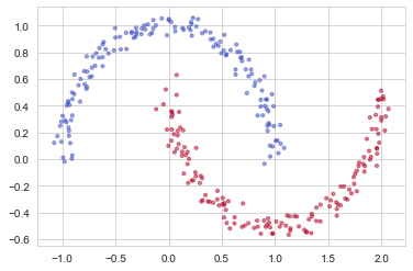
You would like a classifier to separate the blue dots from the red dots.
1 - Neural Network model
You will use a 3-layer neural network (already implemented for you). Here are the initialization methods you will experiment with:
- Zeros initialization – setting
initialization = "zeros"in the input argument. - Random initialization – setting
initialization = "random"in the input argument. This initializes the weights to large random values. - He initialization – setting
initialization = "he"in the input argument. This initializes the weights to random values scaled according to a paper by He et al., 2015.
Instructions: Please quickly read over the code below, and run it. In the next part you will implement the three initialization methods that this model() calls.
def model(X, Y, learning_rate=0.01, num_iterations=15000, print_cost=True, initialization="he"):
    """
    Implements a three-layer neural network: LINEAR->RELU->LINEAR->RELU->LINEAR->SIGMOID.

    Arguments:
    X -- input data, of shape (2, number of examples)
    Y -- true "label" vector (containing 0 for red dots; 1 for blue dots), of shape (1, number of examples)
    learning_rate -- learning rate for gradient descent
    num_iterations -- number of iterations to run gradient descent
    print_cost -- if True, print the cost every 1000 iterations
    initialization -- flag to choose which initialization to use ("zeros","random" or "he")

    Returns:
    parameters -- parameters learnt by the model
    """

    grads = {}
    costs = [] # to keep track of the loss
    m = X.shape[1] # number of examples
    layers_dims = [X.shape[0], 10, 5, 1]

    # Initialize parameters dictionary.
    if initialization == "zeros":
        parameters = initialize_parameters_zeros(layers_dims)
    elif initialization == "random":
        parameters = initialize_parameters_random(layers_dims)
    elif initialization == "he":
        parameters = initialize_parameters_he(layers_dims)

    # Loop (gradient descent)

    for i in range(0, num_iterations):

        # Forward propagation: LINEAR -> RELU -> LINEAR -> RELU -> LINEAR -> SIGMOID.
        a3, cache = forward_propagation(X, parameters)

        # Loss
        cost = compute_loss(a3, Y)

        # Backward propagation.
        grads = backward_propagation(X, Y, cache)

        # Update parameters.
        parameters = update_parameters(parameters, grads, learning_rate)

        # Print the loss every 1000 iterations
        if print_cost and i % 1000 == 0:
            print("Cost after iteration {}: {}".format(i, cost))
            costs.append(cost)

    # plot the loss
    plt.plot(costs)
    plt.ylabel('cost')
    plt.xlabel('iterations (per hundreds)')
    plt.title("Learning rate =" + str(learning_rate))
    plt.show()

    return parameters
2 - Zero initialization
There are two types of parameters to initialize in a neural network:
- the weight matrices \((W^{[1]}, W^{[2]}, W^{[3]}, ..., W^{[L-1]}, W^{[L]})\)
- the bias vectors \((b^{[1]}, b^{[2]}, b^{[3]}, ..., b^{[L-1]}, b^{[L]})\)
Exercise: Implement the following function to initialize all parameters to zeros. You’ll see later that this does not work well since it fails to “break symmetry”, but lets try it anyway and see what happens. Use np.zeros((..,..)) with the correct shapes.
# GRADED FUNCTION: initialize_parameters_zeros

def initialize_parameters_zeros(layers_dims):
    """
    Arguments:
    layer_dims -- python array (list) containing the size of each layer.

    Returns:
    parameters -- python dictionary containing your parameters "W1", "b1", ..., "WL", "bL":
                    W1 -- weight matrix of shape (layers_dims[1], layers_dims[0])
                    b1 -- bias vector of shape (layers_dims[1], 1)
                    ...
                    WL -- weight matrix of shape (layers_dims[L], layers_dims[L-1])
                    bL -- bias vector of shape (layers_dims[L], 1)
    """

    parameters = {}
    L = len(layers_dims)            # number of layers in the network

    for l in range(1, L):
        ### START CODE HERE ### (≈ 2 lines of code)
        parameters['W' + str(l)] = np.zeros((layers_dims[l], layers_dims[l - 1]))
        parameters['b' + str(l)] = np.zeros((layers_dims[l], 1))
        ### END CODE HERE ###
    return parameters
parameters = initialize_parameters_zeros([3,2,1])
print("W1 = " + str(parameters["W1"]))
print("b1 = " + str(parameters["b1"]))
print("W2 = " + str(parameters["W2"]))
print("b2 = " + str(parameters["b2"]))
W1 = [[0. 0. 0.]
 [0. 0. 0.]]
b1 = [[0.]
 [0.]]
W2 = [[0. 0.]]
b2 = [[0.]]
Expected Output:
| **W1** | [[ 0. 0. 0.] [ 0. 0. 0.]] |
| **b1** | [[ 0.] [ 0.]] |
| **W2** | [[ 0. 0.]] |
| **b2** | [[ 0.]] |
Run the following code to train your model on 15,000 iterations using zeros initialization.
plt.subplots(1,1,figsize=(6,4))
parameters = model(train_X, train_Y, initialization = "zeros")
print ("On the train set:")
predictions_train = predict(train_X, train_Y, parameters)
print ("On the test set:")
predictions_test = predict(test_X, test_Y, parameters)
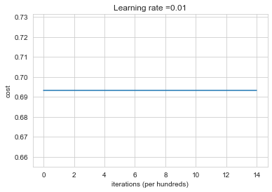
Cost after iteration 0: 0.6931471805599453
Cost after iteration 1000: 0.6931471805599453
Cost after iteration 2000: 0.6931471805599453
Cost after iteration 3000: 0.6931471805599453
Cost after iteration 4000: 0.6931471805599453
Cost after iteration 5000: 0.6931471805599453
Cost after iteration 6000: 0.6931471805599453
Cost after iteration 7000: 0.6931471805599453
Cost after iteration 8000: 0.6931471805599453
Cost after iteration 9000: 0.6931471805599453
Cost after iteration 10000: 0.6931471805599455
Cost after iteration 11000: 0.6931471805599453
Cost after iteration 12000: 0.6931471805599453
Cost after iteration 13000: 0.6931471805599453
Cost after iteration 14000: 0.6931471805599453
On the train set:
Accuracy: 0.5
On the test set:
Accuracy: 0.5
The performance is really bad, and the cost does not really decrease, and the algorithm performs no better than random guessing. Why? Lets look at the details of the predictions and the decision boundary:
print("predictions_train = " + str(predictions_train))
print("predictions_test = " + str(predictions_test))
predictions_train = [[0 0 0 0 0 0 0 0 0 0 0 0 0 0 0 0 0 0 0 0 0 0 0 0 0 0 0 0 0 0 0 0 0 0 0 0
  0 0 0 0 0 0 0 0 0 0 0 0 0 0 0 0 0 0 0 0 0 0 0 0 0 0 0 0 0 0 0 0 0 0 0 0
  0 0 0 0 0 0 0 0 0 0 0 0 0 0 0 0 0 0 0 0 0 0 0 0 0 0 0 0 0 0 0 0 0 0 0 0
  0 0 0 0 0 0 0 0 0 0 0 0 0 0 0 0 0 0 0 0 0 0 0 0 0 0 0 0 0 0 0 0 0 0 0 0
  0 0 0 0 0 0 0 0 0 0 0 0 0 0 0 0 0 0 0 0 0 0 0 0 0 0 0 0 0 0 0 0 0 0 0 0
  0 0 0 0 0 0 0 0 0 0 0 0 0 0 0 0 0 0 0 0 0 0 0 0 0 0 0 0 0 0 0 0 0 0 0 0
  0 0 0 0 0 0 0 0 0 0 0 0 0 0 0 0 0 0 0 0 0 0 0 0 0 0 0 0 0 0 0 0 0 0 0 0
  0 0 0 0 0 0 0 0 0 0 0 0 0 0 0 0 0 0 0 0 0 0 0 0 0 0 0 0 0 0 0 0 0 0 0 0
  0 0 0 0 0 0 0 0 0 0 0 0]]
predictions_test = [[0 0 0 0 0 0 0 0 0 0 0 0 0 0 0 0 0 0 0 0 0 0 0 0 0 0 0 0 0 0 0 0 0 0 0 0
  0 0 0 0 0 0 0 0 0 0 0 0 0 0 0 0 0 0 0 0 0 0 0 0 0 0 0 0 0 0 0 0 0 0 0 0
  0 0 0 0 0 0 0 0 0 0 0 0 0 0 0 0 0 0 0 0 0 0 0 0 0 0 0 0]]
plt.subplots(1,1,figsize=(6,4))
plt.title("Model with Zeros initialization")
axes = plt.gca()
# axes.set_xlim([-1.5, 1.5])
# axes.set_ylim([-1.5, 1.5])
plot_decision_boundary(lambda x: predict_dec(parameters, x.T), train_X, train_Y)
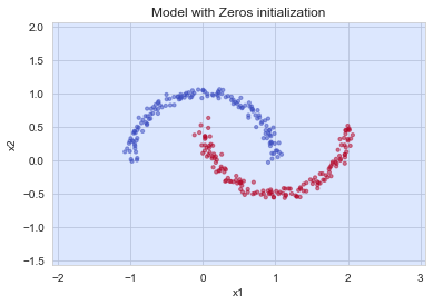
The model is predicting 0 for every example.
In general, initializing all the weights to zero results in the network failing to break symmetry. This means that every neuron in each layer will learn the same thing, and you might as well be training a neural network with \(n^{[l]}=1\) for every layer, and the network is no more powerful than a linear classifier such as logistic regression.
**What you should remember**: - The weights $$W^{[l]}$$ should be initialized randomly to break symmetry. - It is however okay to initialize the biases $$b^{[l]}$$ to zeros. Symmetry is still broken so long as $$W^{[l]}$$ is initialized randomly.3 - Random initialization
To break symmetry, lets intialize the weights randomly. Following random initialization, each neuron can then proceed to learn a different function of its inputs. In this exercise, you will see what happens if the weights are intialized randomly, but to very large values.
Exercise: Implement the following function to initialize your weights to large random values (scaled by *10) and your biases to zeros. Use np.random.randn(..,..) * 10 for weights and np.zeros((.., ..)) for biases. We are using a fixed np.random.seed(..) to make sure your “random” weights match ours, so don’t worry if running several times your code gives you always the same initial values for the parameters.
# GRADED FUNCTION: initialize_parameters_random

def initialize_parameters_random(layers_dims):
    """
    Arguments:
    layer_dims -- python array (list) containing the size of each layer.

    Returns:
    parameters -- python dictionary containing your parameters "W1", "b1", ..., "WL", "bL":
                    W1 -- weight matrix of shape (layers_dims[1], layers_dims[0])
                    b1 -- bias vector of shape (layers_dims[1], 1)
                    ...
                    WL -- weight matrix of shape (layers_dims[L], layers_dims[L-1])
                    bL -- bias vector of shape (layers_dims[L], 1)
    """

    np.random.seed(3)               # This seed makes sure your "random" numbers will be the as ours
    parameters = {}
    L = len(layers_dims)            # integer representing the number of layers

    for l in range(1, L):
        ### START CODE HERE ### (≈ 2 lines of code)
        parameters['W' + str(l)] = np.random.randn(layers_dims[l], layers_dims[l - 1]) * 10
        parameters['b' + str(l)] = np.zeros((layers_dims[l], 1))
        ### END CODE HERE ###

    return parameters
parameters = initialize_parameters_random([3, 2, 1])
print("W1 = " + str(parameters["W1"]))
print("b1 = " + str(parameters["b1"]))
print("W2 = " + str(parameters["W2"]))
print("b2 = " + str(parameters["b2"]))
W1 = [[ 17.88628473   4.36509851   0.96497468]
 [-18.63492703  -2.77388203  -3.54758979]]
b1 = [[0.]
 [0.]]
W2 = [[-0.82741481 -6.27000677]]
b2 = [[0.]]
Expected Output:
| **W1** | [[ 17.88628473 4.36509851 0.96497468] [-18.63492703 -2.77388203 -3.54758979]] |
| **b1** | [[ 0.] [ 0.]] |
| **W2** | [[-0.82741481 -6.27000677]] |
| **b2** | [[ 0.]] |
Run the following code to train your model on 15,000 iterations using random initialization.
plt.subplots(1,1,figsize=(6,4))
parameters = model(train_X, train_Y, initialization = "random")
print("On the train set:")
predictions_train = predict(train_X, train_Y, parameters)
print("On the test set:")
predictions_test = predict(test_X, test_Y, parameters)
<ipython-input-2-c606a8bc266b>:147: RuntimeWarning: divide by zero encountered in log
  logprobs = np.multiply(-np.log(a3),Y) + np.multiply(-np.log(1 - a3), 1 - Y)
<ipython-input-2-c606a8bc266b>:147: RuntimeWarning: invalid value encountered in multiply
  logprobs = np.multiply(-np.log(a3),Y) + np.multiply(-np.log(1 - a3), 1 - Y)


Cost after iteration 0: inf


<ipython-input-2-c606a8bc266b>:19: RuntimeWarning: overflow encountered in exp
  s = 1/(1+np.exp(-x))


Cost after iteration 1000: 1.4689728581497818
Cost after iteration 2000: 0.6422096748947888
Cost after iteration 3000: 0.5183352539690133
Cost after iteration 4000: 0.2980509156122723
Cost after iteration 5000: 0.24392073041135126
Cost after iteration 6000: 0.2424874223607829
Cost after iteration 7000: 0.2421717415715247
Cost after iteration 8000: 0.24260135727310358
Cost after iteration 9000: 0.2428797438736504
Cost after iteration 10000: 0.24221439430112404
Cost after iteration 11000: 0.24156059704466773
Cost after iteration 12000: 0.24091176777584963
Cost after iteration 13000: 0.24026236850861002
Cost after iteration 14000: 0.23959997123320914
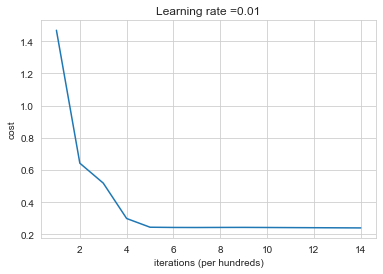
On the train set:
Accuracy: 0.8866666666666667
On the test set:
Accuracy: 0.87
If you see “inf” as the cost after the iteration 0, this is because of numerical roundoff; a more numerically sophisticated implementation would fix this. But this isn’t worth worrying about for our purposes.
Anyway, it looks like you have broken symmetry, and this gives better results. than before. The model is no longer outputting all 0s.
print(predictions_train)
print(predictions_test)
[[1 0 1 1 0 0 0 0 1 1 1 0 1 0 0 0 0 0 1 0 0 0 1 0 0 0 1 0 1 1 0 1 1 0 0 0
  0 0 0 1 1 1 1 1 0 1 1 0 0 1 1 1 1 0 1 0 0 1 1 1 0 0 0 0 0 1 0 0 0 1 1 0
  0 0 0 0 1 0 0 0 0 0 1 0 0 0 1 1 1 1 1 0 0 0 1 0 0 1 1 0 1 0 0 1 0 1 1 0
  0 0 1 1 0 0 0 0 0 1 0 0 1 0 1 0 0 0 0 1 0 1 1 0 0 1 1 1 0 1 1 0 0 0 0 0
  0 0 1 0 1 0 1 0 1 0 1 0 0 0 0 0 1 0 1 1 0 1 0 1 1 0 1 0 1 1 0 1 0 0 1 0
  1 0 0 0 1 0 0 1 1 0 0 1 1 0 0 1 0 1 0 0 1 0 1 1 0 1 1 1 1 0 1 1 1 0 0 1
  0 1 0 0 0 1 0 1 0 0 1 0 0 1 1 0 0 1 0 0 0 0 0 0 0 0 0 0 0 0 0 1 1 0 1 0
  0 1 0 1 1 0 1 0 0 0 0 0 0 0 0 1 0 0 0 1 1 1 1 1 0 0 0 0 1 1 0 0 0 1 1 1
  0 1 1 0 0 0 0 1 1 0 1 0]]
[[1 0 0 0 0 0 0 0 0 0 1 1 1 0 1 0 0 0 1 1 0 0 1 0 1 0 0 1 1 1 1 1 0 0 0 1
  0 1 1 0 0 0 1 0 1 0 0 0 0 0 0 1 0 0 0 0 1 0 1 0 1 1 1 1 1 1 0 0 1 1 1 0
  1 1 1 0 0 0 0 0 0 1 0 0 0 0 1 0 1 1 0 0 0 1 1 0 0 1 0 0]]
plt.subplots(1,1,figsize=(6,4))
plt.title("Model with large random initialization")
axes = plt.gca()
# axes.set_xlim([-1.5, 1.5])
# axes.set_ylim([-1.5, 1.5])
plot_decision_boundary(lambda x: predict_dec(parameters, x.T), train_X, train_Y)
<ipython-input-2-c606a8bc266b>:19: RuntimeWarning: overflow encountered in exp
  s = 1/(1+np.exp(-x))
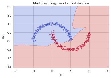
Observations:
- The cost starts very high. This is because with large random-valued weights, the last activation (sigmoid) outputs results that are very close to 0 or 1 for some examples, and when it gets that example wrong it incurs a very high loss for that example. Indeed, when \(\log(a^{[3]}) = \log(0)\), the loss goes to infinity.
- Poor initialization can lead to vanishing/exploding gradients, which also slows down the optimization algorithm.
- If you train this network longer you will see better results, but initializing with overly large random numbers slows down the optimization.
4 - He initialization
Finally, try “He Initialization”; this is named for the first author of He et al., 2015. (If you have heard of “Xavier initialization”, this is similar except Xavier initialization uses a scaling factor for the weights \(W^{[l]}\) of sqrt(1./layers_dims[l-1]) where He initialization would use sqrt(2./layers_dims[l-1]).)
Exercise: Implement the following function to initialize your parameters with He initialization.
Hint: This function is similar to the previous initialize_parameters_random(...). The only difference is that instead of multiplying np.random.randn(..,..) by 10, you will multiply it by \(\sqrt{\frac{2}{\text{dimension of the previous layer}}}\), which is what He initialization recommends for layers with a ReLU activation.
# GRADED FUNCTION: initialize_parameters_he

def initialize_parameters_he(layers_dims):
    """
    Arguments:
    layer_dims -- python array (list) containing the size of each layer.

    Returns:
    parameters -- python dictionary containing your parameters "W1", "b1", ..., "WL", "bL":
                    W1 -- weight matrix of shape (layers_dims[1], layers_dims[0])
                    b1 -- bias vector of shape (layers_dims[1], 1)
                    ...
                    WL -- weight matrix of shape (layers_dims[L], layers_dims[L-1])
                    bL -- bias vector of shape (layers_dims[L], 1)
    """

    np.random.seed(3)
    parameters = {}
    L = len(layers_dims) - 1 # integer representing the number of layers

    for l in range(1, L + 1):
        ### START CODE HERE ### (≈ 2 lines of code)
        parameters['W' + str(l)] = np.random.randn(layers_dims[l], layers_dims[l - 1]) * np.sqrt(2 / layers_dims[l - 1])
        parameters['b' + str(l)] = np.zeros((layers_dims[l], 1))
        ### END CODE HERE ###

    return parameters
parameters = initialize_parameters_he([2, 4, 1])
print("W1 = " + str(parameters["W1"]))
print("b1 = " + str(parameters["b1"]))
print("W2 = " + str(parameters["W2"]))
print("b2 = " + str(parameters["b2"]))
W1 = [[ 1.78862847  0.43650985]
 [ 0.09649747 -1.8634927 ]
 [-0.2773882  -0.35475898]
 [-0.08274148 -0.62700068]]
b1 = [[0.]
 [0.]
 [0.]
 [0.]]
W2 = [[-0.03098412 -0.33744411 -0.92904268  0.62552248]]
b2 = [[0.]]
Expected Output:
| **W1** | [[ 1.78862847 0.43650985] [ 0.09649747 -1.8634927 ] [-0.2773882 -0.35475898] [-0.08274148 -0.62700068]] |
| **b1** | [[ 0.] [ 0.] [ 0.] [ 0.]] |
| **W2** | [[-0.03098412 -0.33744411 -0.92904268 0.62552248]] |
| **b2** | [[ 0.]] |
Run the following code to train your model on 15,000 iterations using He initialization.
plt.subplots(1,1,figsize=(6,4))
parameters = model(train_X, train_Y, initialization = "he")
print("On the train set:")
predictions_train = predict(train_X, train_Y, parameters)
print("On the test set:")
predictions_test = predict(test_X, test_Y, parameters)
Cost after iteration 0: 0.7342482321384683
Cost after iteration 1000: 0.2956649797057583
Cost after iteration 2000: 0.25184038318406815
Cost after iteration 3000: 0.22284974489831486
Cost after iteration 4000: 0.197785000749911
Cost after iteration 5000: 0.17049197570926786
Cost after iteration 6000: 0.13351846788644978
Cost after iteration 7000: 0.09373065428140327
Cost after iteration 8000: 0.06003854894423607
Cost after iteration 9000: 0.0367254088164847
Cost after iteration 10000: 0.023649094476709844
Cost after iteration 11000: 0.016344535872923487
Cost after iteration 12000: 0.011999996046588598
Cost after iteration 13000: 0.009296262994410533
Cost after iteration 14000: 0.00755073011114619
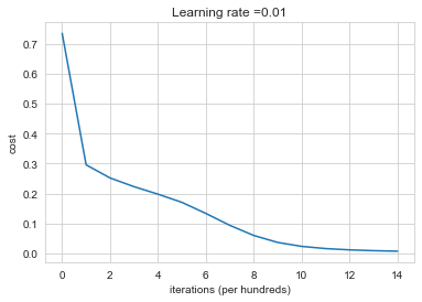
On the train set:
Accuracy: 1.0
On the test set:
Accuracy: 1.0
plt.subplots(1,1,figsize=(6,4))
plt.title("Model with He initialization")
axes = plt.gca()
# axes.set_xlim([-1.5, 1.5])
# axes.set_ylim([-1.5, 1.5])
plot_decision_boundary(lambda x: predict_dec(parameters, x.T), train_X, train_Y)
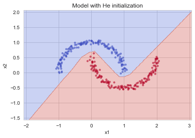
Observations:
- The model with He initialization separates the blue and the red dots very well in a small number of iterations.
5 - Conclusions
You have seen three different types of initializations. For the same number of iterations and same hyperparameters the comparison is:
comparison is:
| Model | Accuracy | Problem |
|---|---|---|
| 3-layer NN with zeros initialization | 50% | Fails to break symmetry |
| 3-layer NN with large random initialization | 83% | Unstable variance |
| 3-layer NN with He initialization | 99% | Normalized variance with 0 mean |
6. Looking at the weight initialization problem from the distribution of activation values
Observing the distribution of the activation value of the hidden layer, we can get a lot of inspiration.
Here, let’s do a simple experiment to see how the initial value of the weight affects the distribution of the activation value of the hidden layer.
Pass in randomly generated input data to a 5-layer neural network (the activation function uses the sigmoid function), and use a histogram to plot the data distribution of the activation values of each layer.
input_data = np.random.randn(1000, 100)  # 1000 data
node_num = 100  # The number of nodes (neurons) in each hidden layer
hidden_layer_size = 5  # There are 5 hidden layers
activations = {}  # The result of activation value is saved here

x = input_data

for i in range(hidden_layer_size):
    if i != 0:
        x = activations[i-1]

    # Change the initial value to experiment!
    w = np.random.randn(node_num, node_num) * 1
    # w = np.random.randn(node_num, node_num) * 0.01
    # w = np.random.randn(node_num, node_num) * np.sqrt(1.0 / node_num)
    # w = np.random.randn(node_num, node_num) * np.sqrt(2.0 / node_num)

    a = np.dot(x, w)
    # Change the type of activation function to experiment!
    z = sigmoid(a)
    # z = ReLU(a)
    # z = tanh(a)

    activations[i] = z

# Draw a histogram
for i, a in activations.items():
    plt.subplot(1, len(activations), i+1)
    plt.title(str(i+1) + "-layer")
    if i != 0: plt.yticks([], [])
    plt.hist(a.flatten(), 30, range=(0,1))
plt.show()
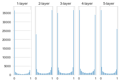
Here it is assumed that the neural network has 5 layers and each layer has 100 units. Then, use Gaussian distribution to randomly generate 1000 data as input data, and pass them to the 5-layer neural network.
The activation values of each layer are distributed towards 0 and 1. The sigmoid function used here is an sigmoid function. As the output continuously approaches 0 (or approaches 1), the value of its derivative gradually approaches 0.
Therefore, the data distribution biased towards 0 and 1 will cause the value of the gradient in the backpropagation to become smaller and eventually disappear. This is the problem of gradient disappearance. In deep learning with deeper levels, the problem of gradient disappearance may be more serious.
Next, set the standard deviation of the weight to 0.01 and implement it again. The code is modified as follows:
for i in range(hidden_layer_size):
    if i != 0:
        x = activations[i-1]

    # Change the initial value to experiment!
    # w = np.random.randn(node_num, node_num) * 1
    w = np.random.randn(node_num, node_num) * 0.01
    # w = np.random.randn(node_num, node_num) * np.sqrt(1.0 / node_num)
    # w = np.random.randn(node_num, node_num) * np.sqrt(2.0 / node_num)

    a = np.dot(x, w)
    # Change the type of activation function to experiment!
    z = sigmoid(a)
    # z = ReLU(a)
    # z = tanh(a)

    activations[i] = z

# Draw a histogram
for i, a in activations.items():
    plt.subplot(1, len(activations), i+1)
    plt.title(str(i+1) + "-layer")
    if i != 0: plt.yticks([], [])
    plt.hist(a.flatten(), 30, range=(0,1))
plt.show()
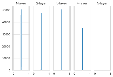
When using a Gaussian distribution with a standard deviation of 0.01, the activation value distribution of each layer is shown in the figure above.
This time concentrate on the distribution around 0.5. Because it is not biased towards 0 and 1 as in the previous example, the problem of vanishing gradient will not occur. However, the distribution of activation values is biased, indicating that there will be a big problem in expressiveness, that is, there is a symmetry problem.
Why do you say that? Because if there are multiple neurons that all output almost the same value, then they have no meaning. For example, if 100 neurons all output almost the same value, then one neuron can also express basically the same thing. Therefore, if the activation value is biased in the distribution, the problem of “restricted expressiveness” will occur.
for i in range(hidden_layer_size):
    if i != 0:
        x = activations[i-1]

    # Change the initial value to experiment!
    # w = np.random.randn(node_num, node_num) * 1
    # w = np.random.randn(node_num, node_num) * 0.01
    w = np.random.randn(node_num, node_num) * np.sqrt(1.0 / node_num)
    # w = np.random.randn(node_num, node_num) * np.sqrt(2.0 / node_num)

    a = np.dot(x, w)
    # Change the type of activation function to experiment!
    z = sigmoid(a)
    # z = ReLU(a)
    # z = tanh(a)

    activations[i] = z

# Draw a histogram
for i, a in activations.items():
    plt.subplot(1, len(activations), i+1)
    plt.title(str(i+1) + "-layer")
    if i != 0: plt.yticks([], [])
    plt.hist(a.flatten(), 30, range=(0,1))
plt.show()
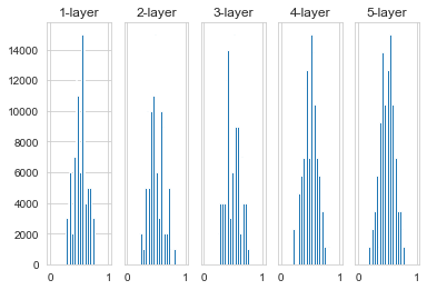
The result after using Xavier’s initial value is shown in the figure above. It can be seen from the image that the more behind the layer, the more skewed the image becomes, but it presents a wider distribution than before. Because the data passed between the layers has an appropriate breadth, the expressive power of the sigmoid function is not limited, and it is expected to be efficient learning.
Because the sigmoid function and the tanh function are symmetrical, the initial value of Xavier is suitable. But when the activation function uses ReLU, it is generally recommended to use the initial value of He.
Now let’s look at the distribution of activation values when the activation function uses ReLU. We have given three reals, which are the results when the initial value of the weight is a Gaussian distribution with a standard deviation of 0.01, when the initial value is the initial value of Xavier, and the initial value is the initial value of He dedicated to ReLU.
Also modify the drawing parameters below to see more clearly:
for i in range(hidden_layer_size):
    if i != 0:
        x = activations[i-1]

    # Change the initial value to experiment!
    # w = np.random.randn(node_num, node_num) * 1
    # w = np.random.randn(node_num, node_num) * 0.01
    # w = np.random.randn(node_num, node_num) * np.sqrt(1.0 / node_num)
    w = np.random.randn(node_num, node_num) * np.sqrt(2.0 / node_num)

    a = np.dot(x, w)
    # Change the type of activation function to experiment!
    # z = sigmoid(a)
    z = relu(a)
    # z = tanh(a)

    activations[i] = z

# Draw a histogram
for i, a in activations.items():
    plt.subplot(1, len(activations), i+1)
    plt.title(str(i+1) + "-layer")
    if i != 0: plt.yticks([], [])
    plt.hist(a.flatten(), 30, range=(0,1))
plt.show()
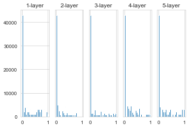
Observing the above figure, we can see that when the standard deviation is a Gaussian distribution of 0.01, the activation value of each layer is very small. The value passed on the neural network is very small, indicating that the gradient of the weight is also very small during back propagation. This is a very serious problem. In fact, there is basically no progress in learning.
Next is the result when the initial value is the initial value of Xavier. In this case, as the layer deepens, the bias becomes a little bit larger. In fact, after the layer is deepened, the bias of the activation value becomes larger, and the problem of the gradient disappears during learning.
When the initial value is the initial value of He, the breadth of distribution in each layer is the same. Since the breadth of the data can remain the same even if the layer is deepened, the appropriate value will be transmitted during the reverse propagation.

Leave a comment