Regression2 (Overfitting and Regularization)

10 minute read

1. Overfitting

import warnings
warnings.filterwarnings(action='ignore') # ignore errors

# 1. magic for inline plot
# 2. magic to print version
# 3. magic so that the notebook will reload external python modules
# 4. magic to enable retina (high resolution) plots
# https://gist.github.com/minrk/3301035
%matplotlib inline
%load_ext watermark
%load_ext autoreload
%autoreload
%config InlineBackend.figure_format = 'retina'

import numpy as np
import cvxpy as cvx
import matplotlib.pyplot as plt
from sklearn import linear_model

%watermark -a 'Jae H. Choi' -d -t -v -p numpy,cvxpy,matplotlib,sklearn

Jae H. Choi 2020-08-18 20:08:42

CPython 3.8.3
IPython 7.16.1

numpy 1.18.5
cvxpy 1.1.3
matplotlib 3.2.2
sklearn 0.23.1

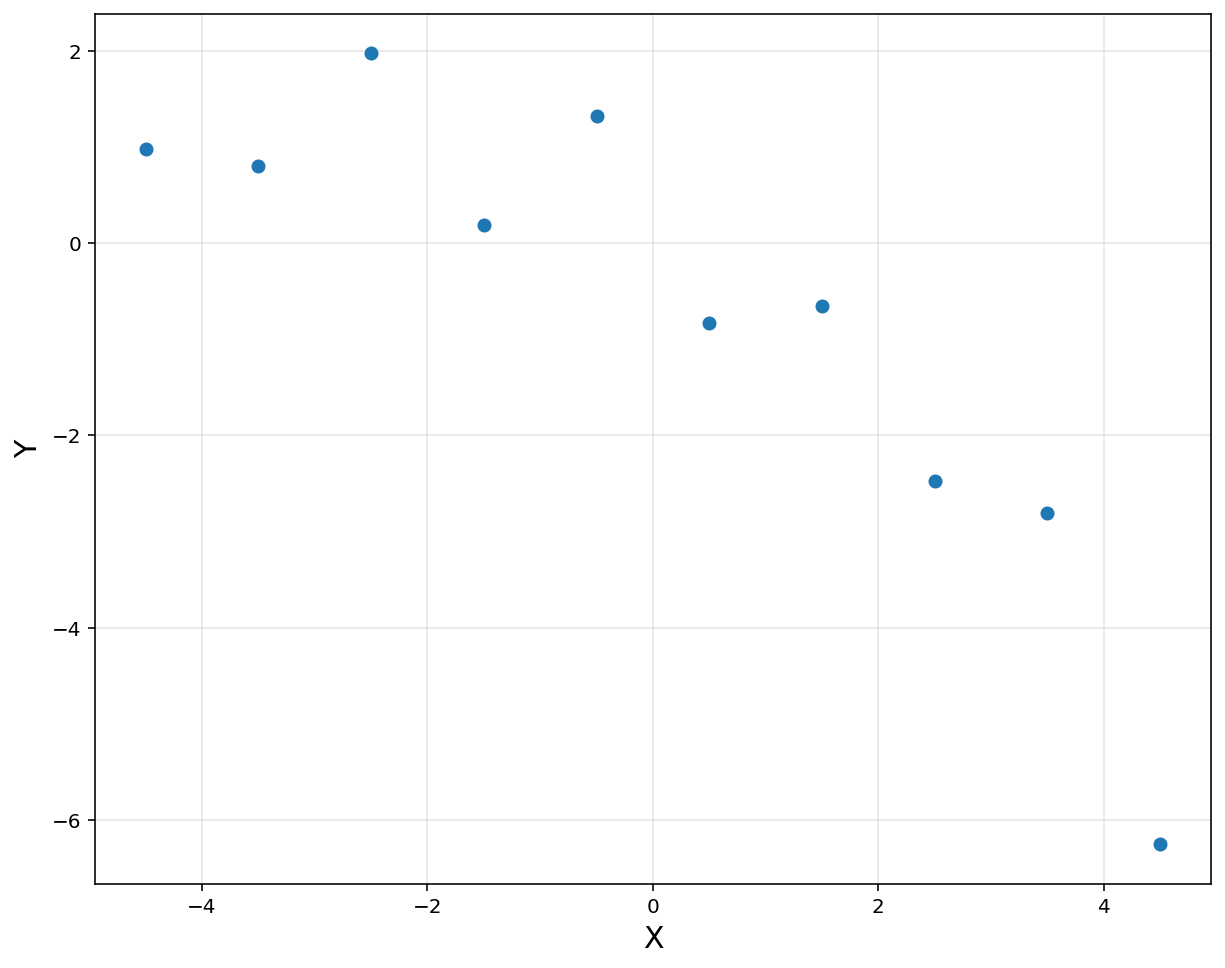
# 10 data points
n = 10
x = np.linspace(-4.5, 4.5, 10).reshape(-1, 1)
y = np.array([0.9819, 0.7973, 1.9737, 0.1838, 1.3180, -0.8361, -0.6591, -2.4701, -2.8122, -6.2512]).reshape(-1, 1)

plt.figure(figsize = (10, 8))
plt.plot(x, y, 'o', label = 'Data')
plt.xlabel('X', fontsize = 15)
plt.ylabel('Y', fontsize = 15)
plt.grid(alpha = 0.3)
plt.show()

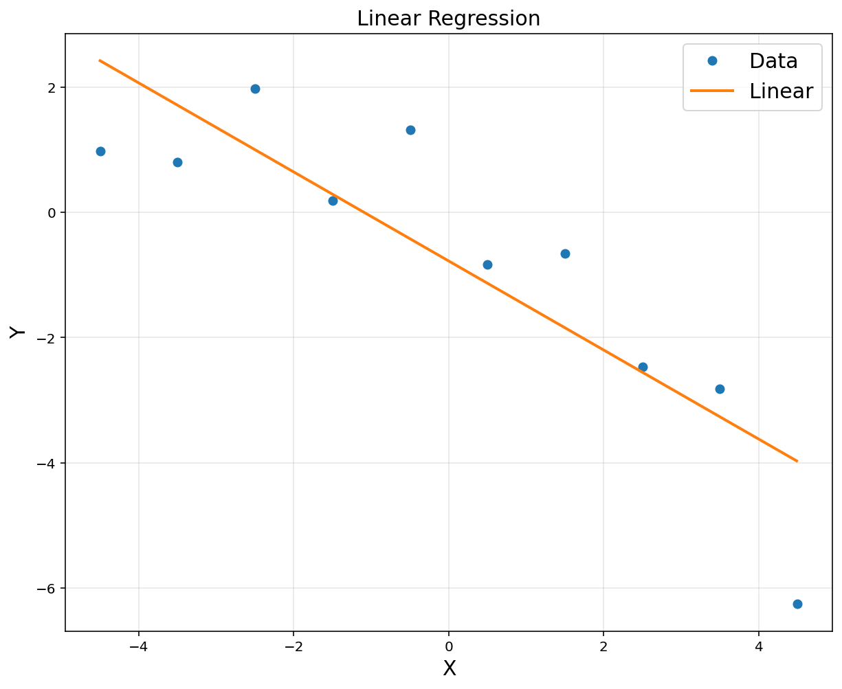
A = np.hstack([x**0, x])
A = np.asmatrix(A)

theta = (A.T*A).I*A.T*y
print(theta)

[[-0.7774    ]
 [-0.71070424]]

# to plot
xp = np.arange(-4.5, 4.5, 0.01).reshape(-1, 1)
yp = theta[0,0] + theta[1,0]*xp

plt.figure(figsize = (10, 8))
plt.plot(x, y, 'o', label = 'Data')
plt.plot(xp[:,0], yp[:,0], linewidth = 2, label = 'Linear')
plt.title('Linear Regression', fontsize = 15)
plt.xlabel('X', fontsize = 15)
plt.ylabel('Y', fontsize = 15)
plt.legend(fontsize = 15)
plt.grid(alpha = 0.3)
plt.show()

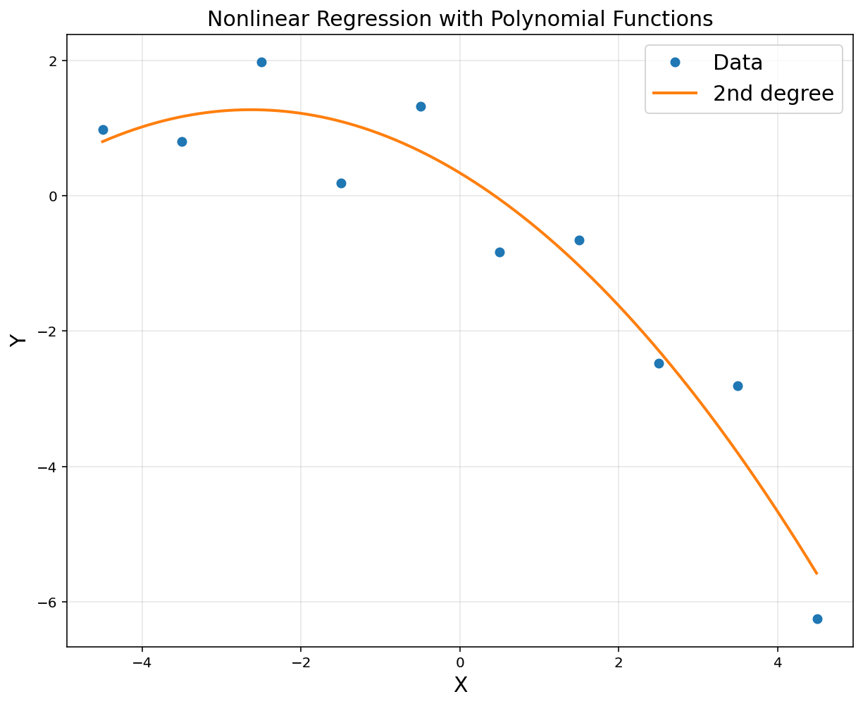
A = np.hstack([x**0, x, x**2])
A = np.asmatrix(A)

theta = (A.T*A).I*A.T*y
print(theta)

[[ 0.33669062]
 [-0.71070424]
 [-0.13504129]]

# to plot
xp = np.arange(-4.5, 4.5, 0.01).reshape(-1, 1)
yp = theta[0,0] + theta[1,0]*xp + theta[2,0]*xp**2

plt.figure(figsize = (10, 8))
plt.plot(x, y, 'o', label = 'Data')
plt.plot(xp[:,0], yp[:,0], linewidth = 2, label = '2nd degree')
plt.title('Nonlinear Regression with Polynomial Functions', fontsize = 15)
plt.xlabel('X', fontsize = 15)
plt.ylabel('Y', fontsize = 15)
plt.legend(fontsize = 15)
plt.grid(alpha = 0.3)
plt.show()

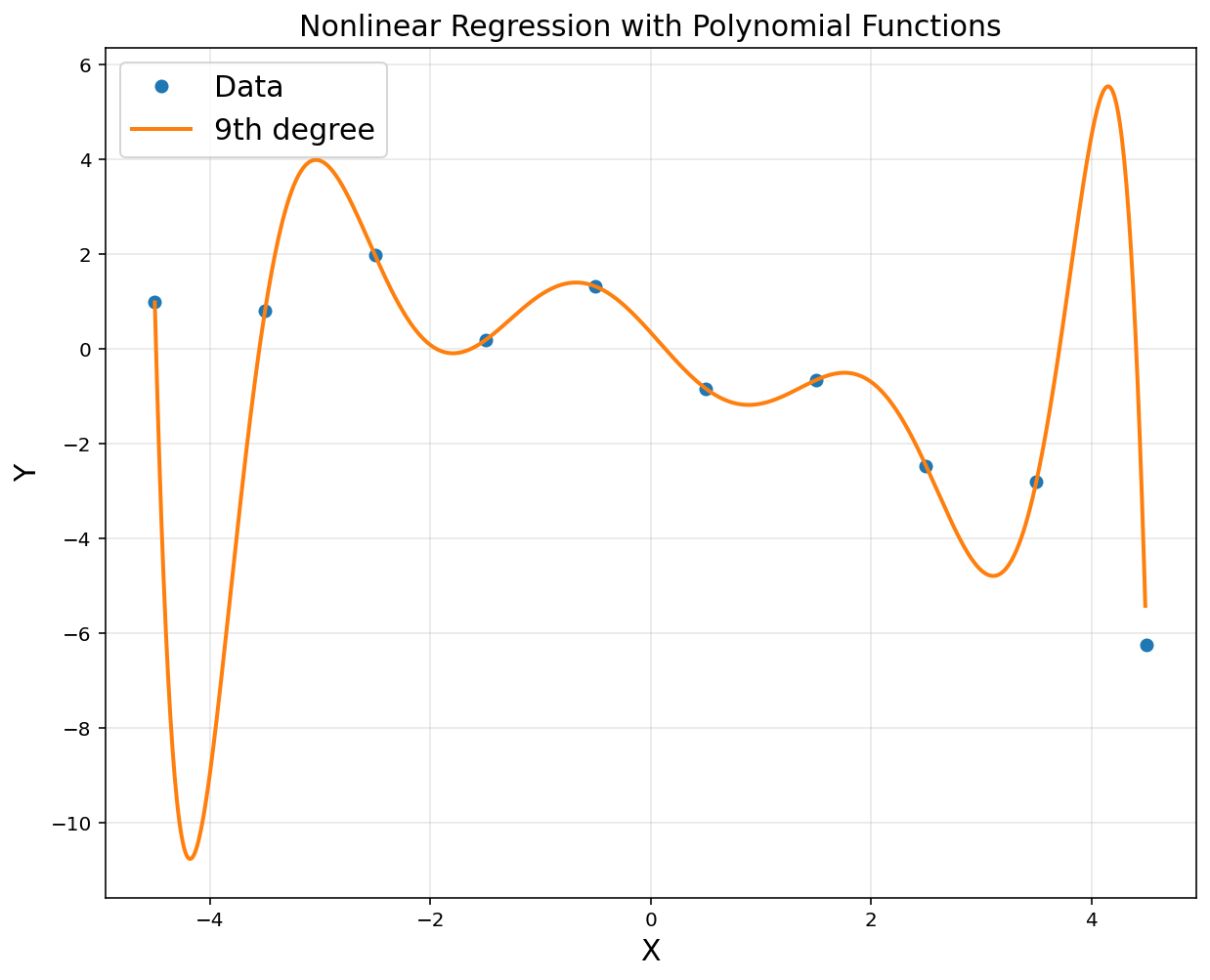
A = np.hstack([x**i for i in range(10)])
A = np.asmatrix(A)
theta = (A.T*A).I*A.T*y
print(theta)
# to plot
xp = np.arange(-4.5, 4.5, 0.01).reshape(-1, 1)

polybasis = np.hstack([xp**i for i in range(10)])
polybasis = np.asmatrix(polybasis)

yp = polybasis*theta

plt.figure(figsize = (10, 8))
plt.plot(x, y, 'o', label = 'Data')
plt.plot(xp[:,0], yp[:,0], linewidth = 2, label = '9th degree')
plt.title('Nonlinear Regression with Polynomial Functions', fontsize = 15)
plt.xlabel('X', fontsize = 15)
plt.ylabel('Y', fontsize = 15)
plt.legend(fontsize = 15)
plt.grid(alpha = 0.3)
plt.show()

[[ 3.48274701e-01]
 [-2.58951123e+00]
 [-4.55286474e-01]
 [ 1.85022226e+00]
 [ 1.06250369e-01]
 [-4.43328786e-01]
 [-9.25753472e-03]
 [ 3.63088178e-02]
 [ 2.35143849e-04]
 [-9.24099978e-04]]

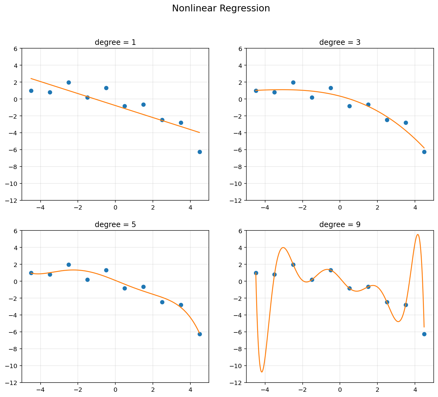
d = [1, 3, 5, 9]
RSS = []

plt.figure(figsize = (12, 10))
plt.suptitle('Nonlinear Regression', fontsize = 15)

for k in range(4):
    A = np.hstack([x**i for i in range(d[k]+1)])
    polybasis = np.hstack([xp**i for i in range(d[k]+1)])

    A = np.asmatrix(A)
    polybasis = np.asmatrix(polybasis)

    theta = (A.T*A).I*A.T*y
    yp = polybasis*theta

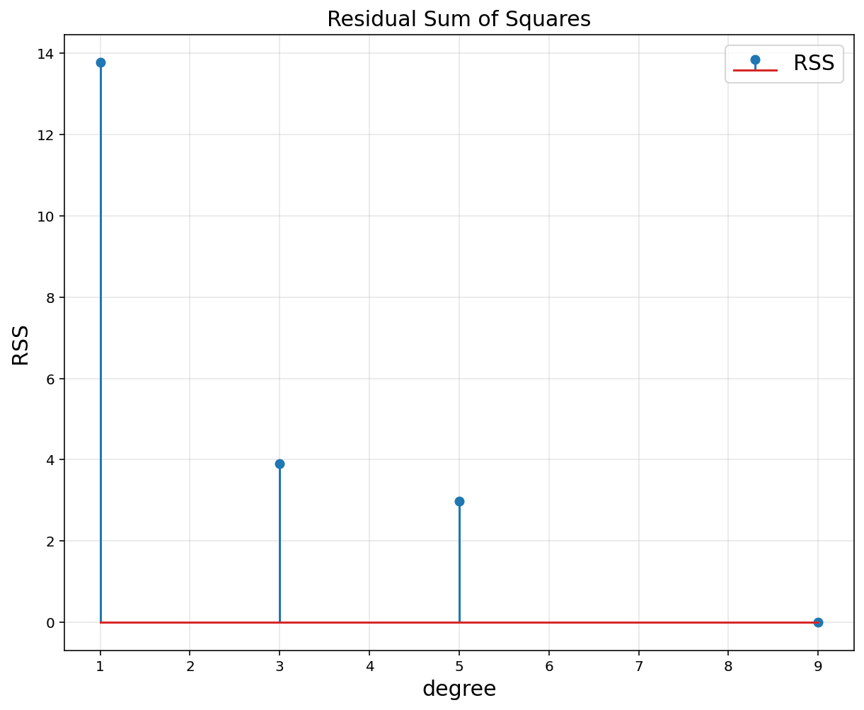
    RSS.append(np.linalg.norm(y - A*theta, 2)**2)

    plt.subplot(2, 2, k+1)
    plt.plot(x, y, 'o')
    plt.plot(xp, yp)
    plt.axis([-5, 5, -12, 6])
    plt.title('degree = {}'.format(d[k]))
    plt.grid(alpha=0.3)

plt.show()

plt.figure(figsize = (10, 8))
plt.stem(d, RSS, label = 'RSS')
plt.title('Residual Sum of Squares', fontsize = 15)
plt.xlabel('degree', fontsize = 15)
plt.ylabel('RSS', fontsize = 15)
plt.legend(fontsize = 15)
plt.grid(alpha = 0.3)
plt.show()

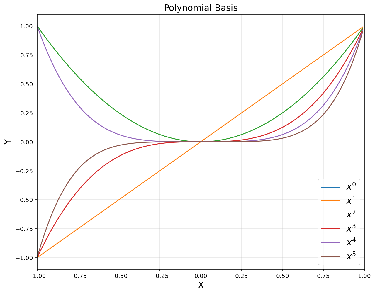
2. Linear Basis Function Models

Construct explicit feature vectors
Consider linear combinations of fixed nonlinear functions of the input variables, of the form

\[\begin{bmatrix} 1 \ x_{1} \ x_1^2\\1 \ x_{2} \ x_2^2\\\vdots \ \vdots\\1 \ x_{m} \ x_m^2 \end{bmatrix} \begin{bmatrix}\theta_0\\\theta_1 \\ \theta_2 \end{bmatrix} \quad \Rightarrow \quad \begin{bmatrix} \mid \ \mid \ \mid \\ b_0(x) \ b_1(x) \ b_2(x)\\ \mid \ \mid \ \mid \end{bmatrix} \begin{bmatrix}\theta_0\\\theta_1 \\ \theta_2 \end{bmatrix}\] \[\hat{y}=\sum_{i=0}^d{\theta_i b_i(x)} = \Phi \ \theta\]

1) Polynomial functions

\[b_i(x) = x^i, \quad i = 0,\cdots,d\]

xp = np.arange(-1, 1, 0.01).reshape(-1, 1)
polybasis = np.hstack([xp**i for i in range(6)])

plt.figure(figsize = (10, 8))

for i in range(6):
    plt.plot(xp, polybasis[:,i], label = '$$x^{}$$'.format(i))

plt.title('Polynomial Basis', fontsize = 15)
plt.xlabel('X', fontsize = 15)
plt.ylabel('Y', fontsize = 15)
plt.axis([-1, 1, -1.1, 1.1])
plt.grid(alpha = 0.3)
plt.legend(fontsize = 15)
plt.show()

2) RBF functions With bandwidth \(\sigma\) and \(k\) RBF centers \(\mu_i \in \mathbb{R}^n\)

\[b_i(x) = \exp \left( - \frac{\lVert x-\mu_i \rVert^2}{2\sigma^2}\right)\]

d = 9

u = np.linspace(-1, 1, d)
sigma = 0.2

rbfbasis = np.hstack([np.exp(-(xp-u[i])**2/(2*sigma**2)) for i in range(d)])

plt.figure(figsize = (10, 8))

for i in range(d):
    plt.plot(xp, rbfbasis[:,i], label='$$\mu = {}$$'.format(u[i]))

plt.title('RBF basis', fontsize = 15)
plt.xlabel('X', fontsize = 15)
plt.ylabel('Y', fontsize = 15)
plt.axis([-1, 1, -0.1, 1.1])
plt.legend(loc = 'lower right', fontsize = 15)
plt.grid(alpha = 0.3)
plt.show()

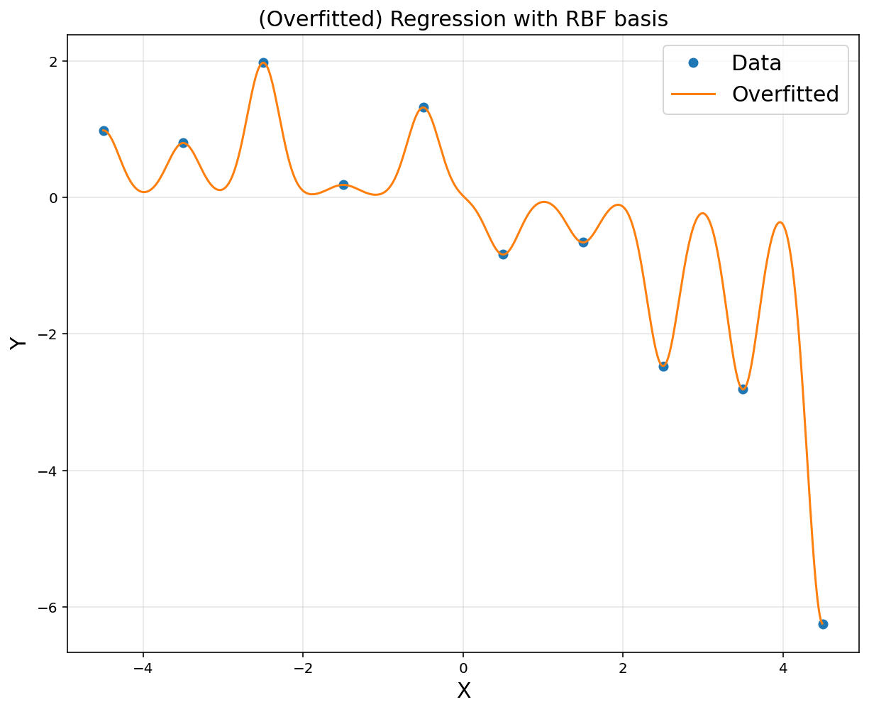
With many features, our prediction function becomes very expressive
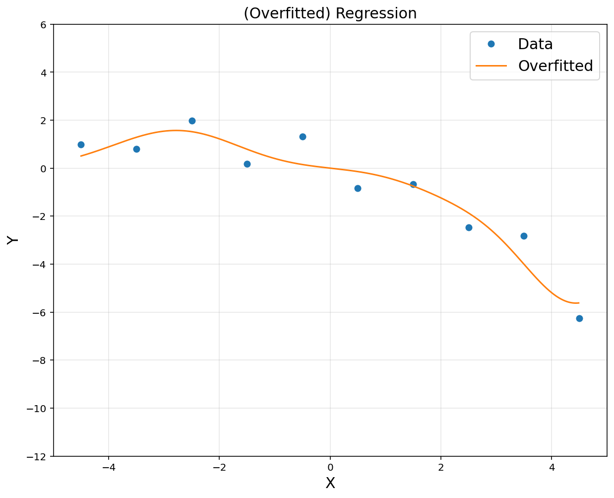
Can lead to overfitting (low error on input data points, but high error nearby)

xp = np.arange(-4.5, 4.5, 0.01).reshape(-1, 1)

d = 10
u = np.linspace(-4.5, 4.5, d)
sigma = 0.2

A = np.hstack([np.exp(-(x-u[i])**2/(2*sigma**2)) for i in range(d)])
rbfbasis = np.hstack([np.exp(-(xp-u[i])**2/(2*sigma**2)) for i in range(d)])

A = np.asmatrix(A)
rbfbasis = np.asmatrix(rbfbasis)

theta = (A.T*A).I*A.T*y
yp = rbfbasis*theta

plt.figure(figsize = (10, 8))
plt.plot(x, y, 'o', label = 'Data')
plt.plot(xp, yp, label = 'Overfitted')
plt.title('(Overfitted) Regression with RBF basis', fontsize = 15)
plt.xlabel('X', fontsize = 15)
plt.ylabel('Y', fontsize = 15)
plt.grid(alpha = 0.3)
plt.legend(fontsize = 15)
plt.show()

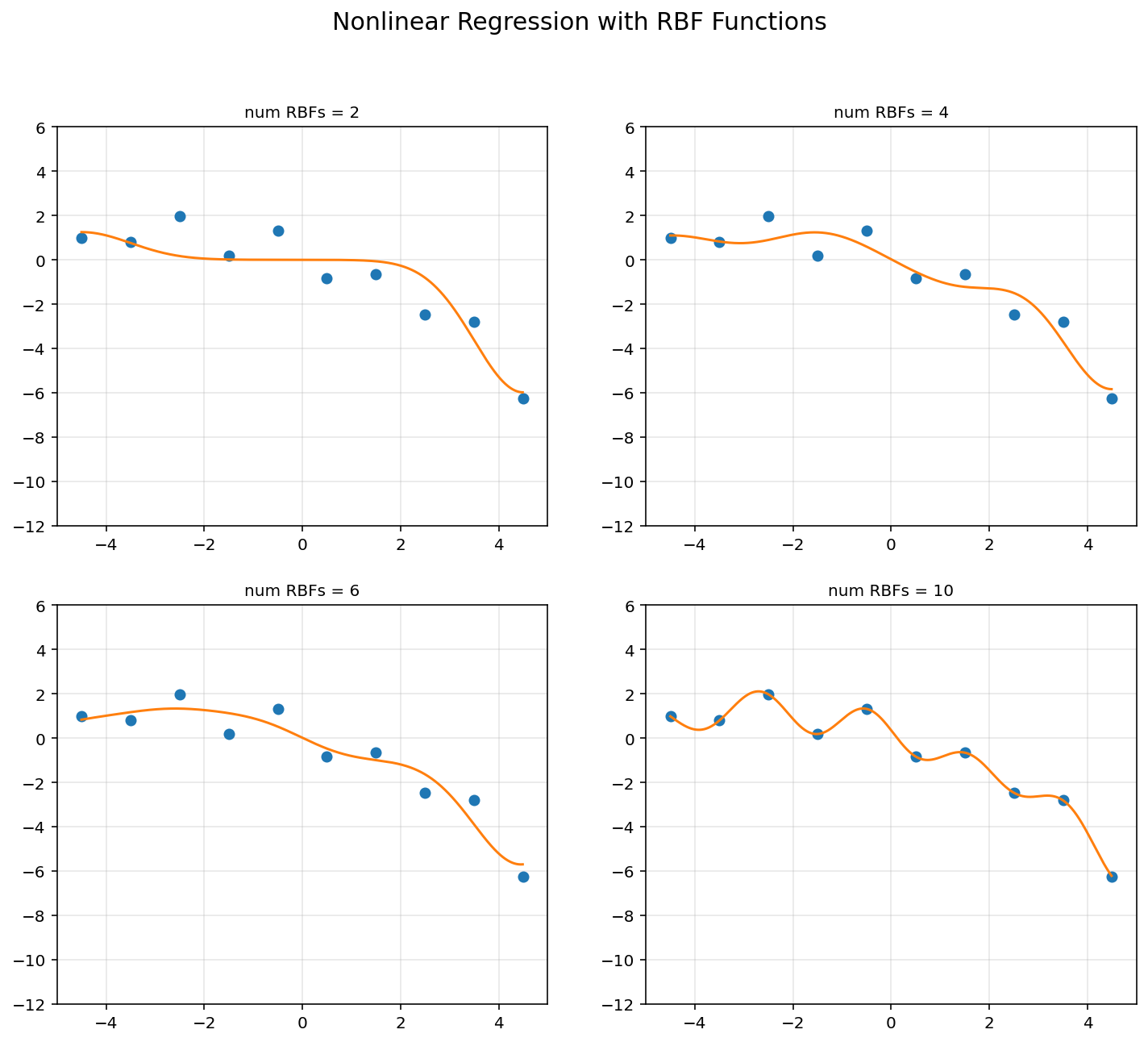
d = [2, 4, 6, 10]
sigma = 1

plt.figure(figsize = (12, 10))
for k in range(4):
    u = np.linspace(-4.5, 4.5, d[k])

    A = np.hstack([np.exp(-(x-u[i])**2/(2*sigma**2)) for i in range(d[k])])
    rbfbasis = np.hstack([np.exp(-(xp-u[i])**2/(2*sigma**2)) for i in range(d[k])])

    A = np.asmatrix(A)
    rbfbasis = np.asmatrix(rbfbasis)

    theta = (A.T*A).I*A.T*y
    yp = rbfbasis*theta

    plt.subplot(2, 2, k+1)
    plt.plot(x, y, 'o')
    plt.plot(xp, yp)
    plt.axis([-5, 5, -12, 6])
    plt.title('num RBFs = {}'.format(d[k]), fontsize = 10)
    plt.grid(alpha = 0.3)

plt.suptitle('Nonlinear Regression with RBF Functions', fontsize = 15)
plt.show()

3. Regularization (Shrinkage Methods)

Often, overfitting associated with very large estimated parameters \(\theta\) We want to balance

how well function fits data
magnitude of coefficients

\[\begin{align*} \text{Total cost } = \; \ \underbrace{\text{measure of fit}}_{RSS(\theta)} + \;\lambda \cdot \underbrace{\text{measure of magnitude of coefficients}}_{\lambda \cdot \lVert \theta \rVert_2^2} \\ \\ \implies \ \min\; \lVert \Phi \theta - y \rVert_2^2 + \lambda \lVert \theta \rVert_2^2 \end{align*}\]

where \(RSS(\theta) = \lVert \Phi\theta - y \rVert^2_2\), ( = Rresidual Sum of Squares) and \(\lambda\) is a tuning parameter to be determined separately

the second term, \(\lambda \cdot \lVert \theta \rVert_2^2\), called a shrinkage penalty, is small when \(\theta_1, \cdots,\theta_d\) are close to zeros, and so it has the effect of shrinking the estimates of \(\theta_j\) towards zero
The tuning parameter \(\lambda\) serves to control the relative impact of these two terms on the regression coefficient estimates
known as a ridge regression
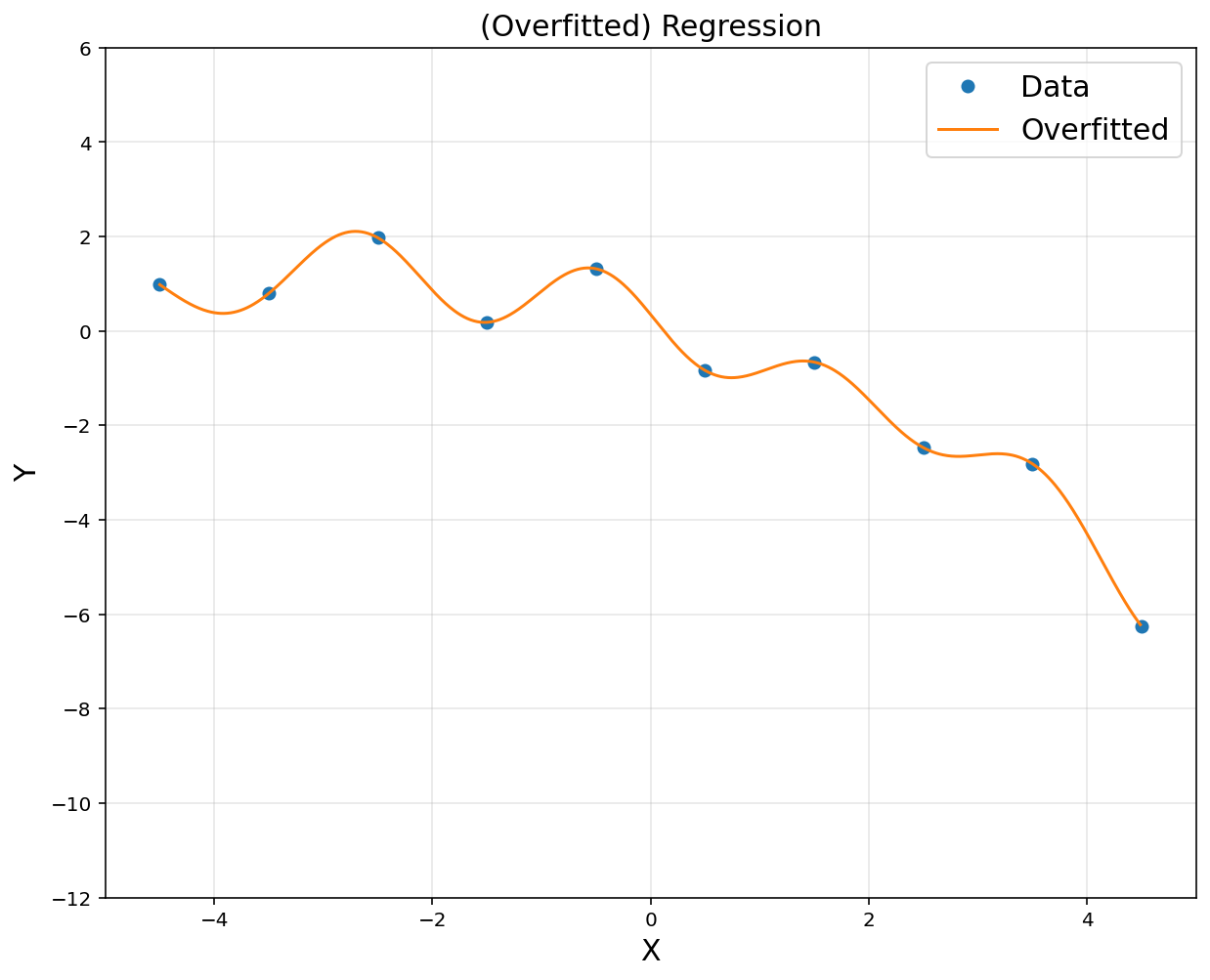
Example: start from rich representation.

\[\min\; \lVert \Phi \theta - y \rVert_2^2\]

# CVXPY code: import cvxpy as cvx
d = 10
u = np.linspace(-4.5, 4.5, d)

sigma = 1
# power(expr, p)
A = np.hstack([np.exp(-(x-u[i])**2/(2*sigma**2)) for i in range(d)])
rbfbasis = np.hstack([np.exp(-(xp-u[i])**2/(2*sigma**2)) for i in range(d)])
A = np.asmatrix(A)
rbfbasis = np.asmatrix(rbfbasis)

theta = cvx.Variable([d, 1])
obj = cvx.Minimize(cvx.sum_squares(A@theta-y))
prob = cvx.Problem(obj).solve()

yp = rbfbasis*theta.value

plt.figure(figsize = (10, 8))
plt.plot(x, y, 'o', label = 'Data')
plt.plot(xp, yp, label = 'Overfitted')
plt.title('(Overfitted) Regression', fontsize = 15)
plt.xlabel('X', fontsize = 15)
plt.ylabel('Y', fontsize = 15)
plt.axis([-5, 5, -12, 6])
plt.legend(fontsize = 15)
plt.grid(alpha = 0.3)
plt.show()

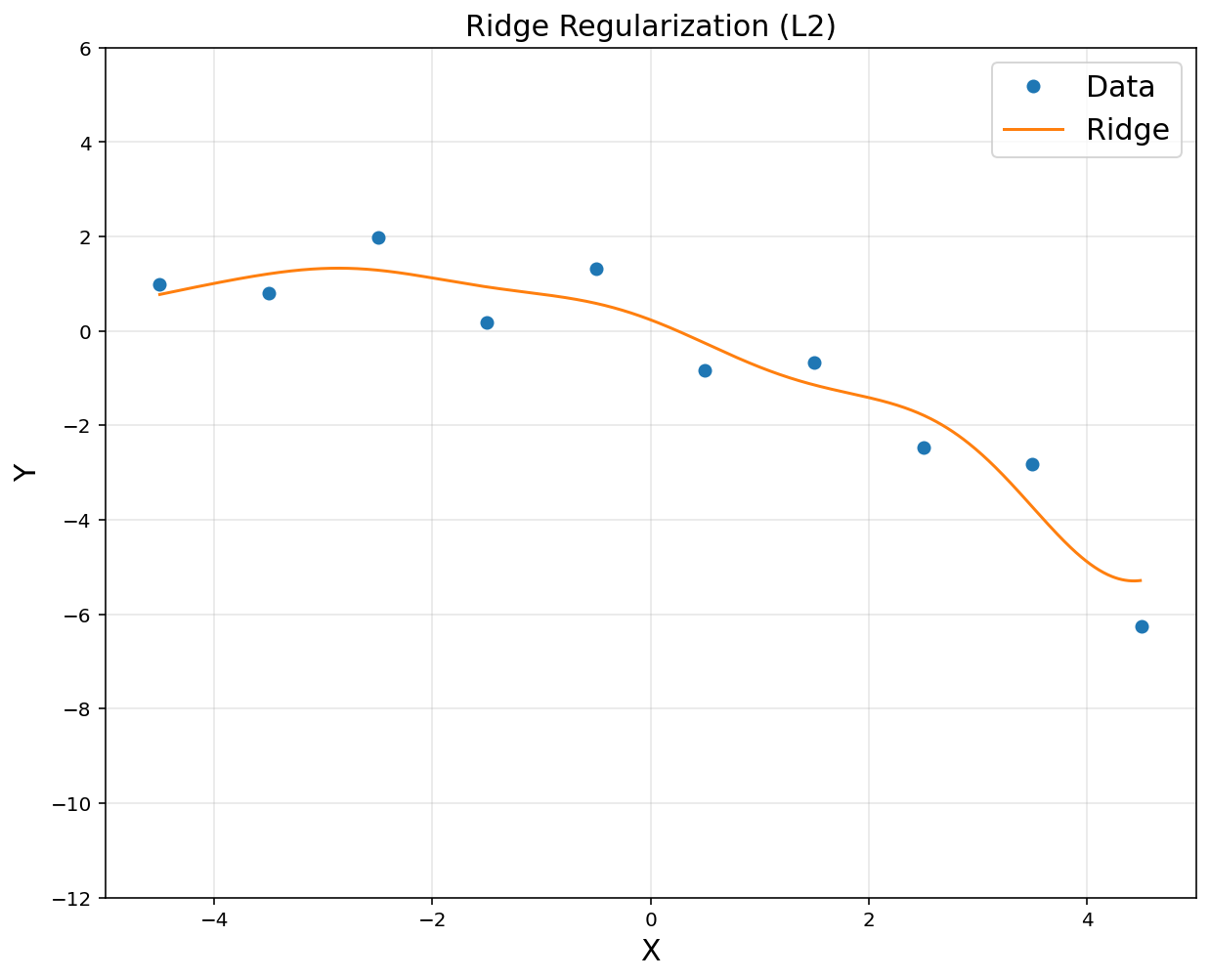
Start from rich representation. Then, regularize coefficients \(\theta\)

\[\min\; \lVert \Phi \theta - y \rVert_2^2 + \lambda \lVert \theta \rVert_2^2\]

# ridge regression
lamb = 0.1
theta = cvx.Variable([d, 1])
obj = cvx.Minimize(cvx.sum_squares(A@theta - y) + lamb*cvx.sum_squares(theta))
prob = cvx.Problem(obj).solve()

yp = rbfbasis*theta.value

plt.figure(figsize = (10, 8))
plt.plot(x, y, 'o', label = 'Data')
plt.plot(xp, yp, label = 'Ridge')
plt.title('Ridge Regularization (L2)', fontsize = 15)
plt.xlabel('X', fontsize = 15)
plt.ylabel('Y', fontsize = 15)
plt.axis([-5, 5, -12, 6])
plt.legend(fontsize = 15)
plt.grid(alpha = 0.3)
plt.show()

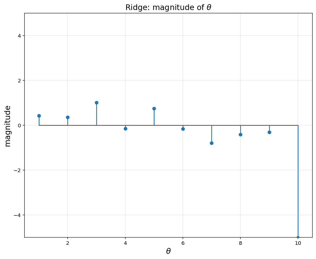
# Regulization (= ridge nonlinear regression) encourages small weights, but not exactly 0
plt.figure(figsize = (10, 8))
plt.title(r'Ridge: magnitude of $$\theta$$', fontsize = 15)
plt.xlabel(r'$$\theta$$', fontsize = 15)
plt.ylabel('magnitude', fontsize = 15)
plt.stem(np.linspace(1, 10, 10).reshape(-1, 1), theta.value)
plt.xlim([0.5, 10.5])
plt.ylim([-5, 5])
plt.grid(alpha = 0.3)
plt.show()

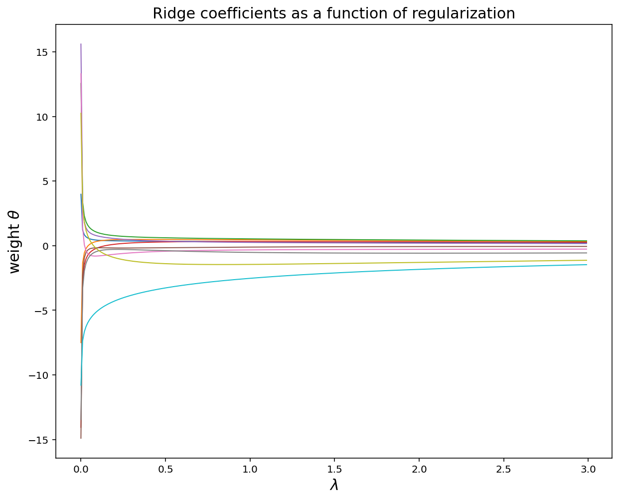
lamb = np.arange(0,3,0.01)

theta_record = []
for k in lamb:
    theta = cvx.Variable([d, 1])
    obj = cvx.Minimize(cvx.sum_squares(A@theta - y) + k*cvx.sum_squares(theta))
    prob = cvx.Problem(obj).solve()
    theta_record.append(np.ravel(theta.value))

plt.figure(figsize = (10, 8))
plt.plot(lamb, theta_record, linewidth = 1)
plt.title('Ridge coefficients as a function of regularization', fontsize = 15)
plt.xlabel('$$\lambda$$', fontsize = 15)
plt.ylabel(r'weight $$\theta$$', fontsize = 15)
plt.show()

4. Sparsity for Feature Selection using LASSO

Least Squares with a penalty on the \(l_1\) norm of the parameters
Start with full model (all possible features)
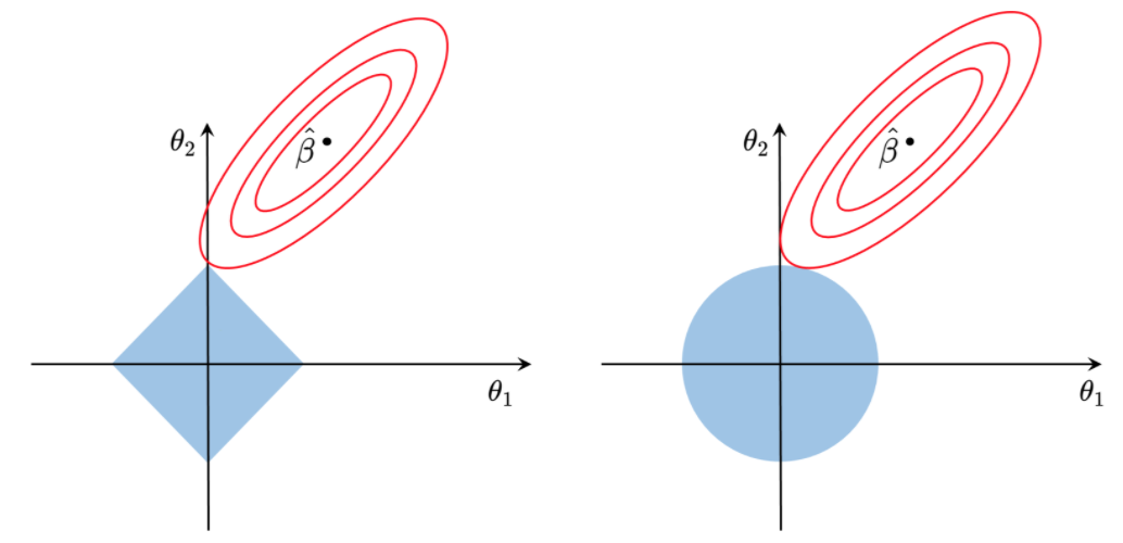
‘Shrink’ some coefficients exactly to 0
- i.e., knock out certain features
- the \(l_1\) penalty has the effect of forcing some of the coefficient estimates to be exactly equal to zero
Non-zero coefficients indicate ‘selected’ features

Try this cost instead of ridge…

\[\begin{align*} \text{Total cost } = \; \ \underbrace{\text{measure of fit}}_{RSS(\theta)} + \;\lambda \cdot \underbrace{\text{measure of magnitude of coefficients}}_{\lambda \cdot \lVert \theta \rVert_1} \\ \\ \implies \ \min\; \lVert \Phi \theta - y \rVert_2^2 + \lambda \lVert \theta \rVert_1 \end{align*}\]

\(\lambda\) is a tuning parameter = balance of fit and sparsity
Another equivalent forms of optimizations

\[\begin{array}{rl} \begin{align*} \min_{\theta} \quad \ \lVert \Phi \theta - y \rVert_2^2 \\ \text{subject to} \quad \ \lVert \theta \rVert_1 \leq s_1 \end{align*} \end{array} \quad\quad\quad\quad \begin{array}{rl} \min_{\theta} \; \ \lVert \Phi \theta - y \rVert_2^2 \\ \text{subject to} \; \ \lVert \theta \rVert_2 \leq s_2 \end{array}\]

\[\min\; \lVert \Phi \theta - y \rVert_2^2 + \lambda \lVert \theta \rVert_1\]

# LASSO regression
lamb = 2
theta = cvx.Variable([d, 1])
obj = cvx.Minimize(cvx.sum_squares(A@theta - y) + lamb*cvx.norm(theta, 1))
prob = cvx.Problem(obj).solve()

yp = rbfbasis@theta.value

plt.figure(figsize = (10, 8))
plt.title('LASSO Regularization (L1)', fontsize = 15)
plt.xlabel('X', fontsize = 15)
plt.ylabel('Y', fontsize = 15)
plt.plot(x, y, 'o', label = 'Data')
plt.plot(xp, yp, label = 'LASSO')
plt.axis([-5, 5, -12, 6])
plt.legend(fontsize = 15)
plt.grid(alpha = 0.3)
plt.show()

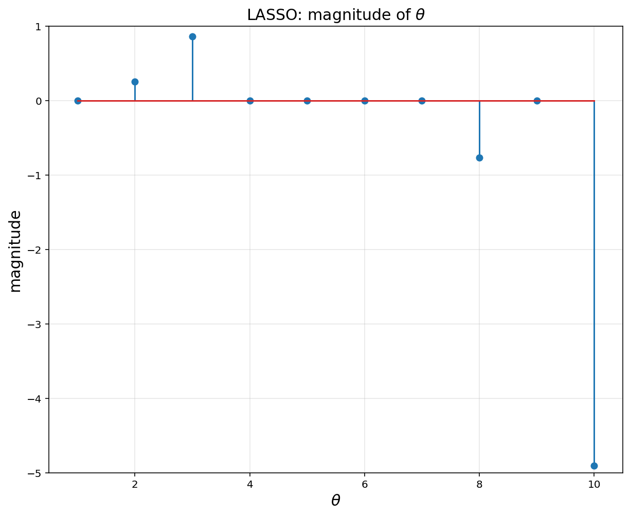
# Regulization (= Lasso nonlinear regression) encourages zero weights
plt.figure(figsize = (10, 8))
plt.title(r'LASSO: magnitude of $$\theta$$', fontsize = 15)
plt.xlabel(r'$$\theta$$', fontsize = 15)
plt.ylabel('magnitude', fontsize = 15)
plt.stem(np.arange(1,11), theta.value)
plt.xlim([0.5, 10.5])
plt.ylim([-5,1])
plt.grid(alpha = 0.3)
plt.show()

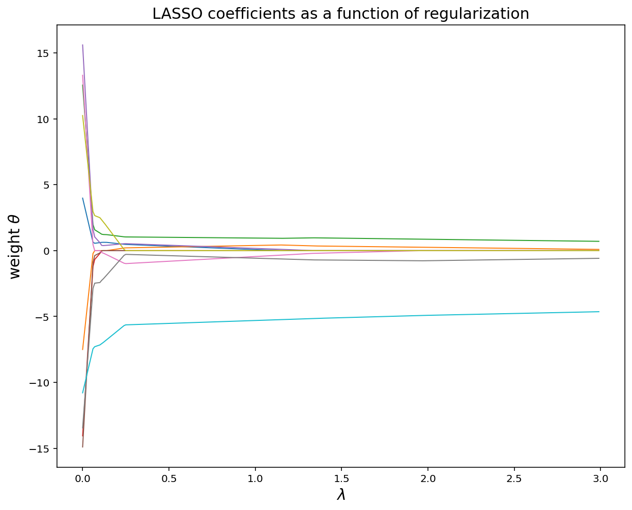
lamb = np.arange(0,3,0.01)
theta_record = []
for k in lamb:
    theta = cvx.Variable([d, 1])
    obj = cvx.Minimize(cvx.sum_squares(A@theta - y) + k*cvx.norm(theta, 1))
    prob = cvx.Problem(obj).solve()
    theta_record.append(np.ravel(theta.value))
plt.figure(figsize = (10, 8))
plt.plot(lamb, theta_record, linewidth = 1)
plt.title('LASSO coefficients as a function of regularization', fontsize = 15)
plt.xlabel('$$\lambda$$', fontsize = 15)
plt.ylabel(r'weight $$\theta$$', fontsize = 15)
plt.show()

# reduced order model
# we will use only theta 2, 3, 8, 10
d = 4
u = np.array([-3.5, -2.5, 2.5, 4.5])

sigma = 1

A = np.hstack([np.exp(-(x-u[i])**2/(2*sigma**2)) for i in range(d)])
rbfbasis = np.hstack([np.exp(-(xp-u[i])**2/(2*sigma**2)) for i in range(d)])

A = np.asmatrix(A)
rbfbasis = np.asmatrix(rbfbasis)

theta = cvx.Variable([d, 1])
obj = cvx.Minimize(cvx.norm(A@theta-y, 2))
prob = cvx.Problem(obj).solve()

yp = rbfbasis@theta.value

plt.figure(figsize = (10, 8))
plt.plot(x, y, 'o', label = 'Data')
plt.plot(xp, yp, label = 'Overfitted')
plt.title('(Overfitted) Regression', fontsize = 15)
plt.xlabel('X', fontsize = 15)
plt.ylabel('Y', fontsize = 15)
plt.axis([-5, 5, -12, 6])
plt.legend(fontsize = 15)
plt.grid(alpha = 0.3)
plt.show()

5. L2 and L1 Regularizers

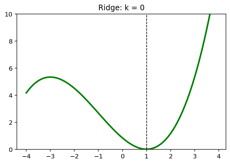
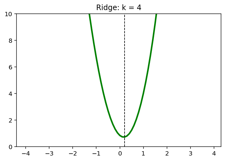
\[\min \;(x-1)^2 + \frac{1}{6}(x-1)\]

5.1. L2 Penality

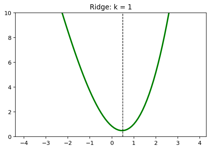
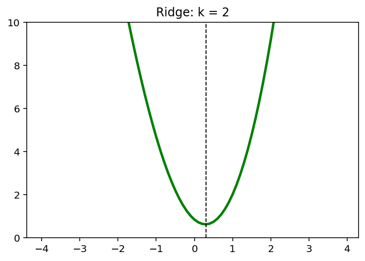
\[\min \; (x-1)^2 + \frac{1}{6}(x-1) + kx^2, \quad k=0,1,2,\cdots\]

x = np.arange(-4,4,0.1)
k = 4
y = (x-1)**2 + 1/6*(x-1)**3 + k*x**2
x_star = x[np.argmin(y)]
print(x_star)

0.20000000000000373

plt.plot(x, y, 'g', linewidth = 2.5)
plt.axvline(x = x_star, color = 'k', linewidth = 1, linestyle = '--')
plt.ylim([0,10])
plt.show()

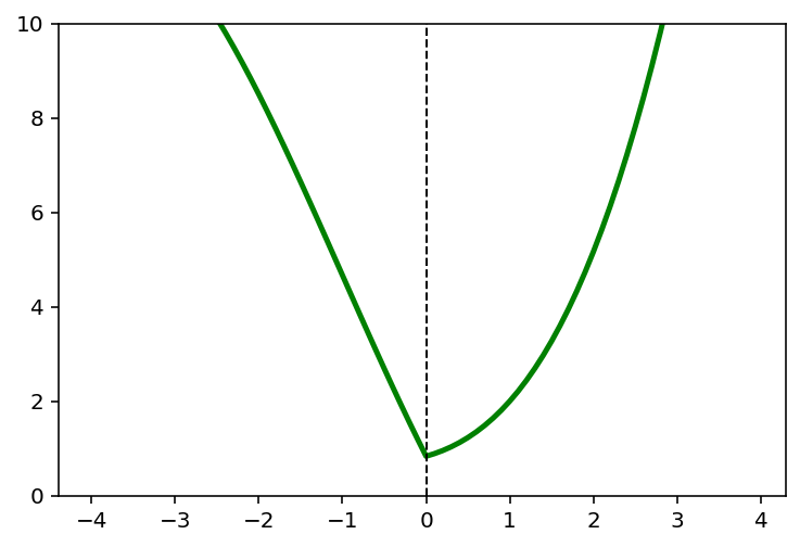
for k in [0,1,2,4]:
    y = (x-1)**2 + 1/6*(x-1)**3 + k*x**2
    x_star = x[np.argmin(y)]

    plt.plot(x,y, 'g', linewidth = 2.5)
    plt.axvline(x = x_star, color = 'k', linewidth = 1, linestyle = '--')
    plt.ylim([0,10])
    plt.title('Ridge: k = {}'.format(k))
    plt.show()

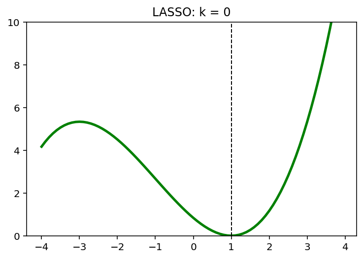
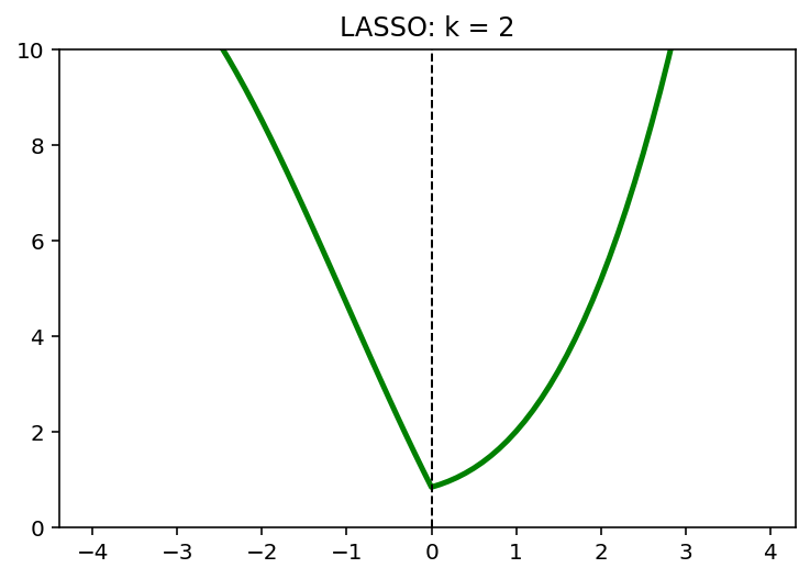
5.2. L1 Penalty

\[\min \; (x-1)^2 + \frac{1}{6}(x-1) + k\lvert x \rvert, \quad k=0,1,2,\cdots\]

x = np.arange(-4,4,0.1)
k = 2
y = (x-1)**2 + 1/6*(x-1)**3 + k*abs(x)

x_star = x[np.argmin(y)]
print(x_star)

3.552713678800501e-15 ```python plt.plot(x, y, 'g', linewidth = 2.5) plt.axvline(x = x_star, color = 'k', linewidth = 1, linestyle = '--') plt.ylim([0,10]) plt.show() ```

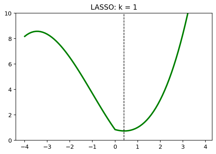
for k in [0,1,2]:
    y = (x-1)**2 + 1/6*(x-1)**3 + k*abs(x)
    x_star = x[np.argmin(y)]

    plt.plot(x,y, 'g', linewidth = 2.5)
    plt.axvline(x = x_star, color = 'k', linewidth = 1, linestyle = '--')
    plt.ylim([0,10])
    plt.title('LASSO: k = {}'.format(k))
    plt.show()

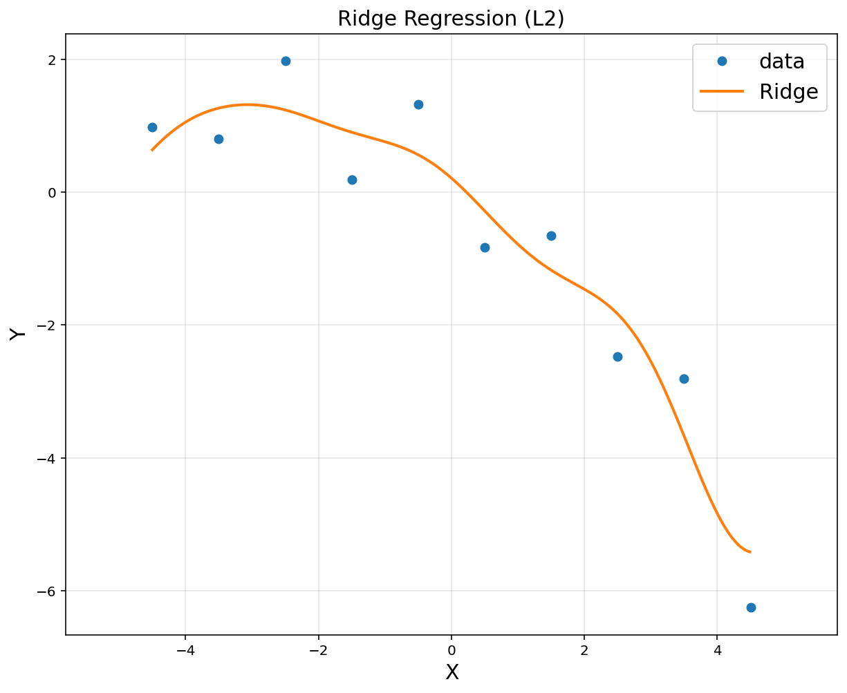
6. Scikit-Learn

RBF functions \(g_i(x)\) as basis

\[\begin{align*} \Phi \ = \begin{bmatrix} \mid \ \mid \ \ \mid \\ b_0(x) \ b_1(x) \ \cdots \ b_d(x) \\ \mid \ \mid \ \ \mid \end{bmatrix} = \begin{bmatrix} 1 \ \mid \ \ \mid \\ \vdots \ b_1(x) \ \cdots \ b_d(x) \\ 1 \ \mid \ \ \mid \end{bmatrix}\\\\ \implies \Phi \theta \ = \sum_{i=0}^d \theta_i b_i(x) : \; \text{a linearly-combined function of RBF basis with coefficients of } \theta \end{align*}\]

# 10 data points
n = 10
x = np.linspace(-4.5, 4.5, 10).reshape(-1, 1)
y = np.array([0.9819, 0.7973, 1.9737, 0.1838, 1.3180, -0.8361, -0.6591, -2.4701, -2.8122, -6.2512]).reshape(-1, 1)
d = 10
u = np.linspace(-4.5, 4.5, d)
sigma = 1
A = np.hstack([np.exp(-(x-u[i])**2/(2*sigma**2)) for i in range(d)])

#from sklearn import linear_model
reg = linear_model.Ridge(alpha = 0.1)
reg.fit(A,y)

Ridge(alpha=0.1)

# to plot
xp = np.arange(-4.5, 4.5, 0.01).reshape(-1, 1)
Ap = np.hstack([np.exp(-(xp-u[i])**2/(2*sigma**2)) for i in range(d)])

plt.figure(figsize = (10, 8))
plt.plot(x, y, 'o', label = "data")
plt.plot(xp, reg.predict(Ap), linewidth = 2, label = "Ridge")
plt.title('Ridge Regression (L2)', fontsize = 15)
plt.xlabel('X', fontsize = 15)
plt.ylabel('Y', fontsize = 15)
plt.legend(fontsize = 15)
plt.axis('equal')
plt.grid(alpha = 0.3)
plt.show()

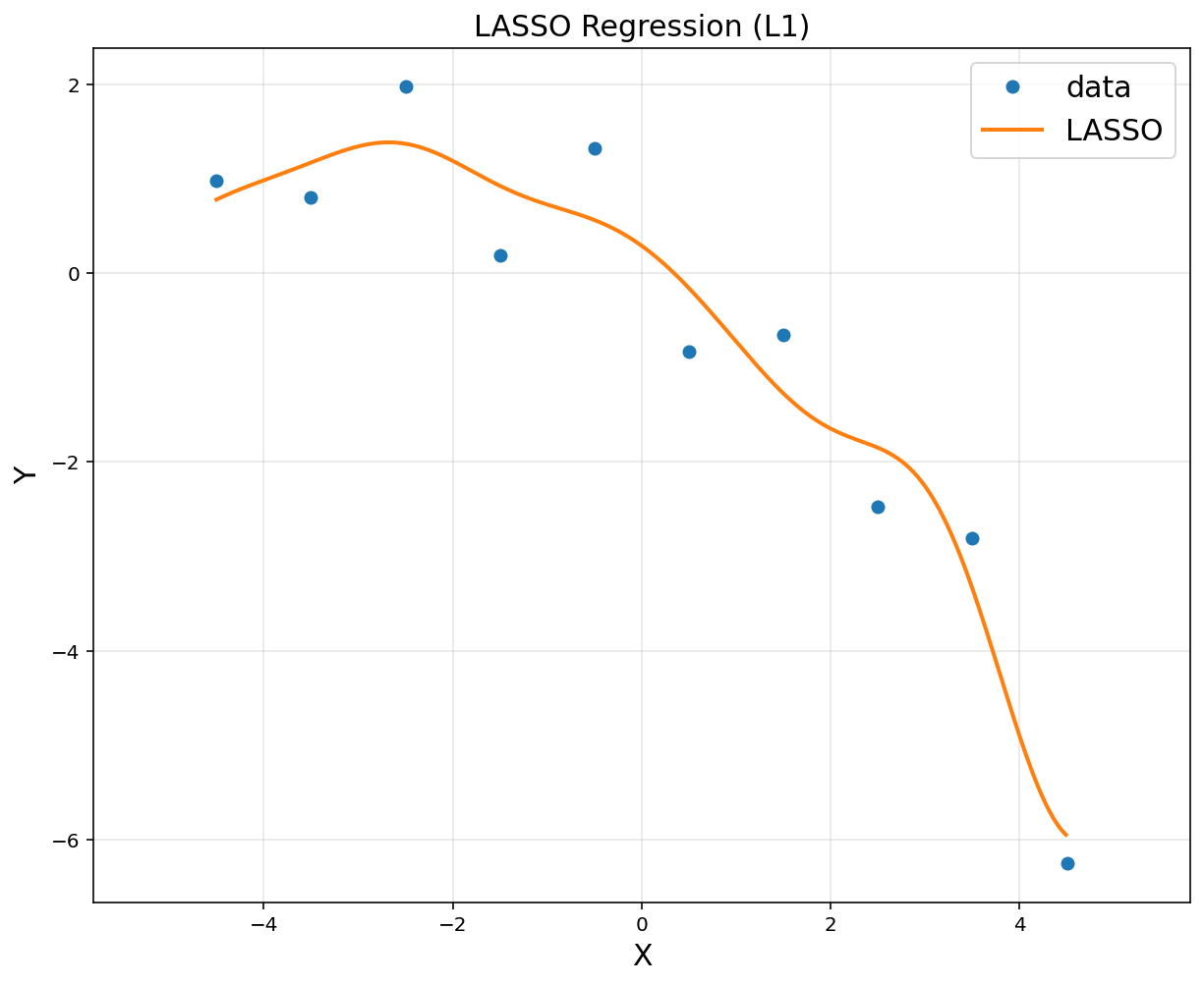
reg = linear_model.Lasso(alpha = 0.005)
reg.fit(A,y)

Lasso(alpha=0.005)

# to plot
xp = np.arange(-4.5, 4.5, 0.01).reshape(-1, 1)
Ap = np.hstack([np.exp(-(xp-u[i])**2/(2*sigma**2)) for i in range(d)])

plt.figure(figsize = (10, 8))
plt.plot(x, y, 'o', label = "data")
plt.plot(xp, reg.predict(Ap), linewidth = 2, label = "LASSO")
plt.title('LASSO Regression (L1)', fontsize = 15)
plt.xlabel('X', fontsize = 15)
plt.ylabel('Y', fontsize = 15)
plt.legend(fontsize = 15)
plt.axis('equal')
plt.grid(alpha = 0.3)
plt.show()

Share on

Twitter Facebook LinkedIn

Jae H. Choi

Regression2 (Overfitting and Regularization)

1. Overfitting

2. Linear Basis Function Models

3. Regularization (Shrinkage Methods)

4. Sparsity for Feature Selection using LASSO

5. L2 and L1 Regularizers

5.1. L2 Penality

5.2. L1 Penalty

6. Scikit-Learn

Share on

Leave a comment

You may also enjoy

Interview Preparation1

Deep Learning Applications in Computer Vision

Deep Learning Performance Improvement 4 - Back-propagation

Deep Learning Performance Improvement 3 - Regularization