
Regression3 (Regression Applications)
Regression Examples
1. De-noising Signal
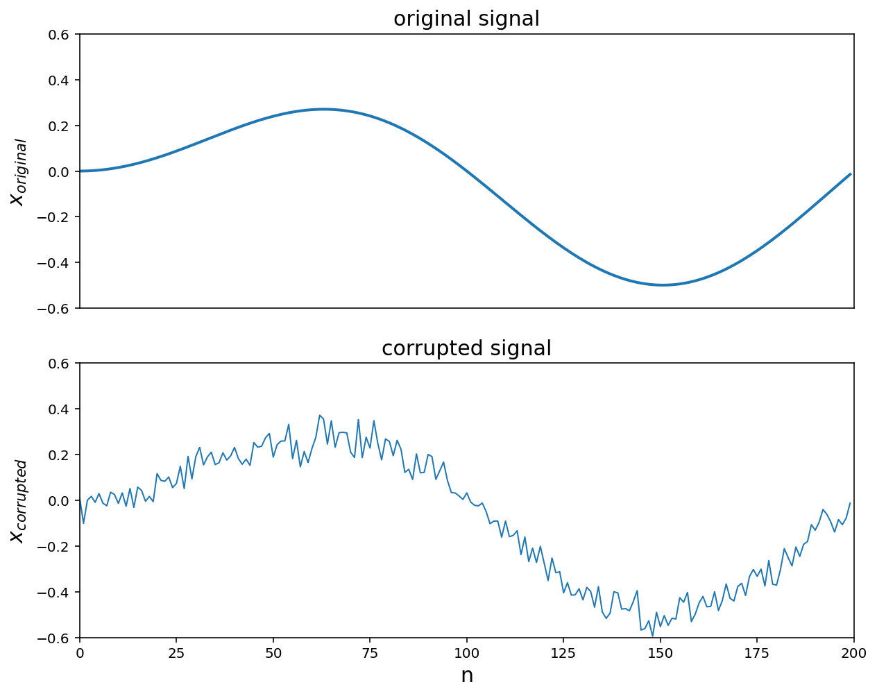
We start with a signal represented by a vector \(x \in \mathbb{R}^n\). The coefficients \(x_i\) correspond to the value of some function of time, evaluated (or sampled, in the language of signal processing) at evenly spaced points. It is usually assumed that the signal does not vary too rapidly, which means that usually, we have \(x_i \approx x_{i+1}\). Suppose we have a signal \(x\), which does not vary too rapidly and that \(x\) is corrupted by some small, rapidly varying noise \(\varepsilon\),
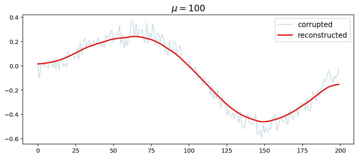
i.e. \(x_{cor} = x + \varepsilon\). Then if we want to reconstruct \(x\) from \(x_{cor}\) we should solve (with \(\hat{x}\) as the parameter)
\[\text{minimize} \quad \lVert \hat{x} - x_{cor}\rVert_2^2 + \mu\sum_{i=1}^{n-1}(x_{i+1}-x_i)^2\]where the parameter \(\mu\) controls the ‘smoothnes’ of \(\hat{x}\).
Source:
- Boyd Vandenberghe’s book
- Figures 6.8-6.10: Quadratic smoothing
- Week 4 of Linear and Integer Programming by Coursera of Univ. of Colorado
# ignore errors
import warnings
warnings.filterwarnings(action='ignore')
# 1. magic for inline plot
# 2. magic to print version
# 3. magic so that the notebook will reload external python modules
# 4. magic to enable retina (high resolution) plots
# https://gist.github.com/minrk/3301035
%matplotlib inline
%load_ext watermark
%load_ext autoreload
%autoreload
%config InlineBackend.figure_format = 'retina'

import numpy as np
import matplotlib.pyplot as plt
import pandas as pd
import cvxpy as cvx
%watermark -a 'Jae H. Choi' -d -t -v -p numpy,pandas,matplotlib,sklearn,cvxpy
Jae H. Choi 2020-08-18 22:57:09

CPython 3.8.3
IPython 7.16.1

numpy 1.18.5
pandas 1.0.5
matplotlib 3.2.2
sklearn 0.23.1
cvxpy 1.1.3
n = 200
t = np.arange(n).reshape(-1,1)
x = 0.5 * np.sin((2*np.pi/n)*t) * (np.sin(0.01*t))
x_cor = x + 0.05*np.random.randn(n,1)

plt.figure(figsize = (10, 8))
plt.subplot(2,1,1)
plt.plot(t,x,'-', linewidth = 2)
plt.axis([0, n, -0.6, 0.6])
plt.xticks([])
plt.title('original signal' , fontsize = 15)
plt.ylabel('$$x_{original}$$', fontsize = 15)

plt.subplot(2,1,2)
plt.plot(t, x_cor,'-', linewidth = 1)
plt.axis([0, n, -0.6, 0.6])
plt.title('corrupted signal', fontsize = 15)
plt.xlabel('n', fontsize = 15)
plt.ylabel('$$x_{corrupted}$$', fontsize = 15)
plt.show()
1.1. Transform de-noising in time into an optimization problem
\[X = \begin{bmatrix} x_{1} \\ x_{2} \\ \vdots \\ x_{n} \end{bmatrix}\] \[\large \min\limits_{X}\;\left\{\underbrace{\lVert(X - X_{cor})\rVert^2_{2}}_{\text{how much } X \text{ deviates from }X_{cor}} + \mu \underbrace{\sum_{k = 1}^{n-1}(x_{k+1}-x_{k})^2}_{\text{penalize rapid changes of } X}\right\}\]- \(\min\limits_{X}\;\lVert(X - X_{cor})\rVert^2_{2}\): \(\quad\) How much \(X\) deviates from \(X_{cor}\)
- \(\mu\sum\limits_{k = 1}^{n-1}(x_{k+1}-x_{k})^2\): \(\quad\) penalize rapid changes of \(X\)
- \(\mu\) : to adjust the relative weight of 1. & 2.
- In a vector form
- \[X - X_{cor} = I_n X - X_{cor}\]
- \(\sum\;(x_{k+1}-x_{k})^2\) :
\(\qquad \qquad\) 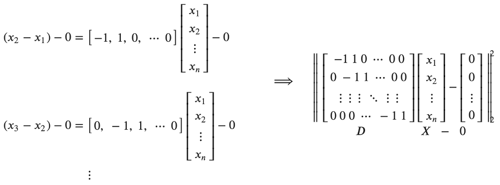
\(\begin{align*} \left\Vert I_n X-X_{cor}\big\Vert^2_{2} + \mu\big\Vert DX-0\right\Vert^2_{2} \ = \big\Vert Ax-b\big\Vert^2_{2} \\ \\ \ = \Bigg\Vert \begin{bmatrix} I_n\\ \sqrt{\mu}D \end{bmatrix} X- \begin{bmatrix} X_{cor}\\ 0 \end{bmatrix} \Bigg\Vert^2_{2} \end{align*}\) \(\text{where} \; A = \begin{bmatrix} I_n\\ \sqrt{\mu}D \end{bmatrix},\quad b = \begin{bmatrix} X_{cor}\\ 0 \end{bmatrix}\)
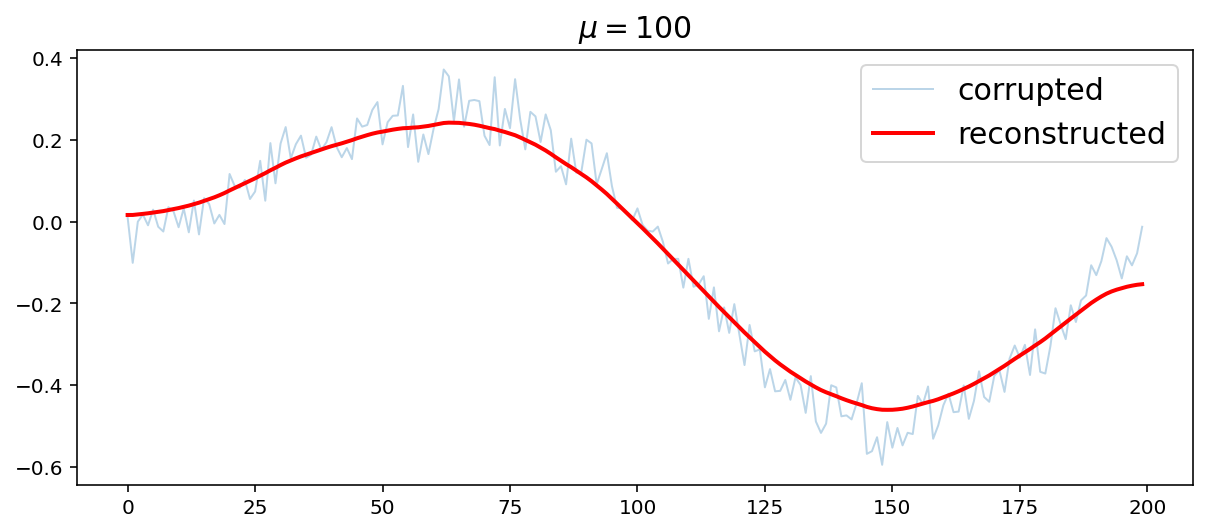
- Then, plug \(A\), \(b\) to \((A^TA)^{-1}A^Tb\)
mu = 100

D = np.zeros([n-1, n])
D[:,0:n-1] -= np.eye(n-1)

D[:,1:n] += np.eye(n-1)
A = np.vstack([np.eye(n), np.sqrt(mu)*D])

b = np.vstack([x_cor, np.zeros([n-1,1])])

A = np.asmatrix(A)
b = np.asmatrix(b)

x_reconst = (A.T*A).I*A.T*b

plt.figure(figsize = (10, 4))
plt.plot(t, x_cor, '-', linewidth = 1, alpha = 0.3, label = 'corrupted');
plt.plot(t, x_reconst, 'r', linewidth = 2, label = 'reconstructed')
plt.title('$$\mu = {}$$'.format(mu), fontsize = 15)
plt.legend(fontsize = 15)
plt.show()
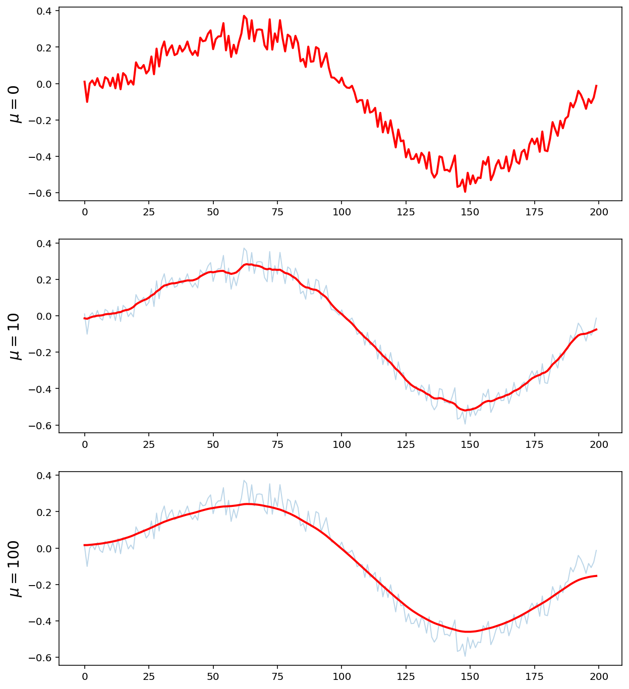
1.2. with different \(\mu\)’s (see how \(\mu\) affects smoothing results)
plt.figure(figsize = (10, 12))

mu = [0, 10, 100];

for i in range(len(mu)):
    A = np.vstack([np.eye(n), np.sqrt(mu[i])*D])
    b = np.vstack([x_cor, np.zeros([n-1,1])])

    A = np.asmatrix(A)
    b = np.asmatrix(b)

    x_reconst = (A.T*A).I*A.T*b

    plt.subplot(3,1,i+1)
    plt.plot(t, x_cor, '-', linewidth = 1, alpha = 0.3)
    plt.plot(t, x_reconst, 'r', linewidth = 2)
    plt.ylabel('$$\mu = {}$$'.format(mu[i]), fontsize = 15)

plt.show()
1.3. CVXPY Implementation
cvxpytoolbox to numerically solve
mu = 100

x_reconst = cvx.Variable([n,1])
#obj = cvx.Minimize(cvx.sum_squares(x_reconst - x_cor) + mu*cvx.sum_squares(x_reconst[1:n]-x_reconst[0:n-1]))
obj = cvx.Minimize(cvx.sum_squares(x_reconst - x_cor) + mu*cvx.sum_squares(D@x_reconst))

prob = cvx.Problem(obj).solve()

plt.figure(figsize = (10, 4))
plt.plot(t, x_cor, '-', linewidth = 1, alpha = 0.3, label = 'corrupted');
plt.plot(t, x_reconst.value, 'r', linewidth = 2, label = 'reconstructed')
plt.title('$$\mu = {}$$'.format(mu), fontsize = 15)
plt.legend(fontsize = 12)
plt.show()
plt.figure(figsize = (10, 12))

mu = [0, 10, 100]

for i in range(len(mu)):
    x_reconst = cvx.Variable([n,1])
    obj = cvx.Minimize(cvx.sum_squares(x_reconst - x_cor) + mu[i]*cvx.sum_squares(D@x_reconst))
    prob = cvx.Problem(obj).solve()

    plt.subplot(3,1,i+1)
    plt.plot(t,x_cor,'-', linewidth = 1, alpha = 0.3)
    plt.plot(t,x_reconst.value, 'r', linewidth = 2)
    plt.ylabel('$$\mu = {}$$'.format(int(mu[i])), fontsize = 15)

plt.show()

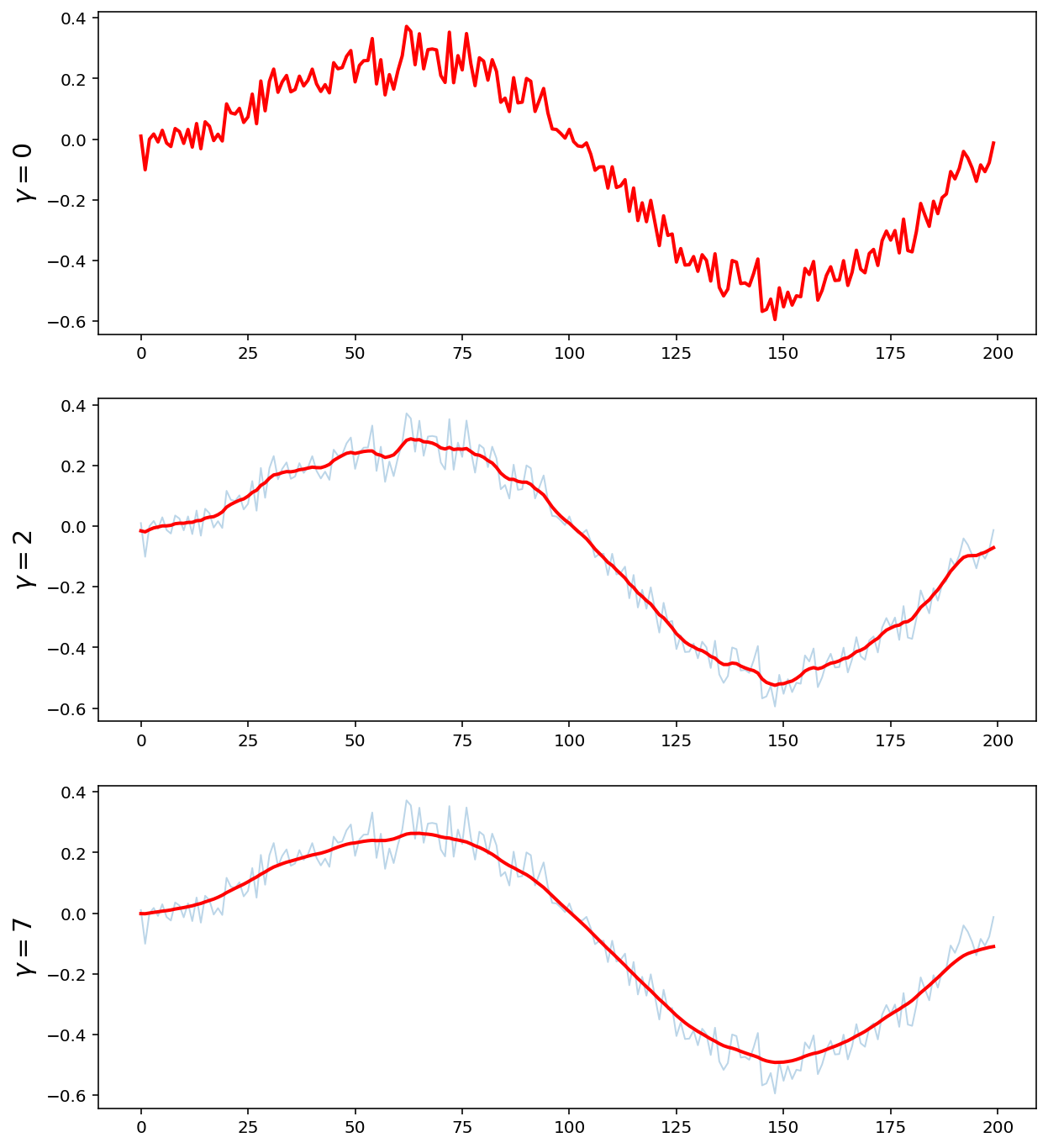
1.4. L2 Norm
-
CVXPY strongly encourages to eliminate quadratic forms, that is, functions like
sum_squares,sum(square(.))orquad_form -
Whenever it is possible to construct equivalent models using
norminstead
plt.figure(figsize = (10, 12))

gammas = [0, 2, 7]

for i in range(len(gammas)):
    x_reconst = cvx.Variable([n,1])
    obj = cvx.Minimize(cvx.norm(x_reconst-x_cor, 2) + gammas[i]*(cvx.norm(D@x_reconst, 2)))
    prob = cvx.Problem(obj).solve()

    plt.subplot(3,1,i+1)
    plt.plot(t,x_cor,'-', linewidth = 1, alpha = 0.3)
    plt.plot(t,x_reconst.value, 'r', linewidth = 2)
    plt.ylabel('$$ \gamma = {}$$'.format(gammas[i]), fontsize = 15)

plt.show()
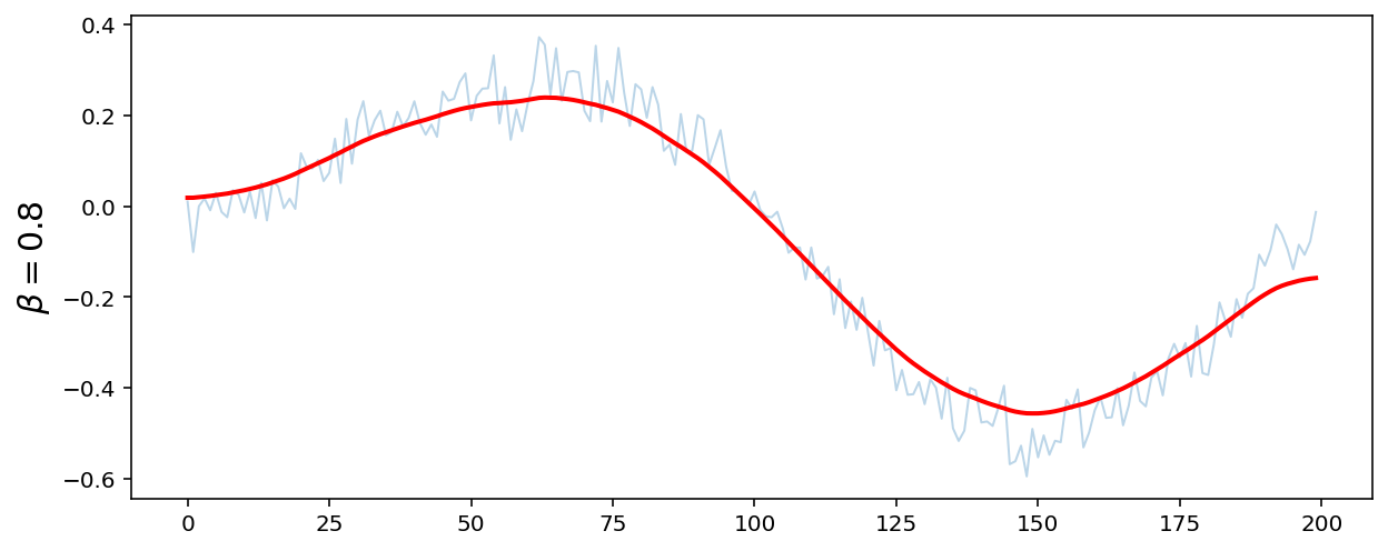
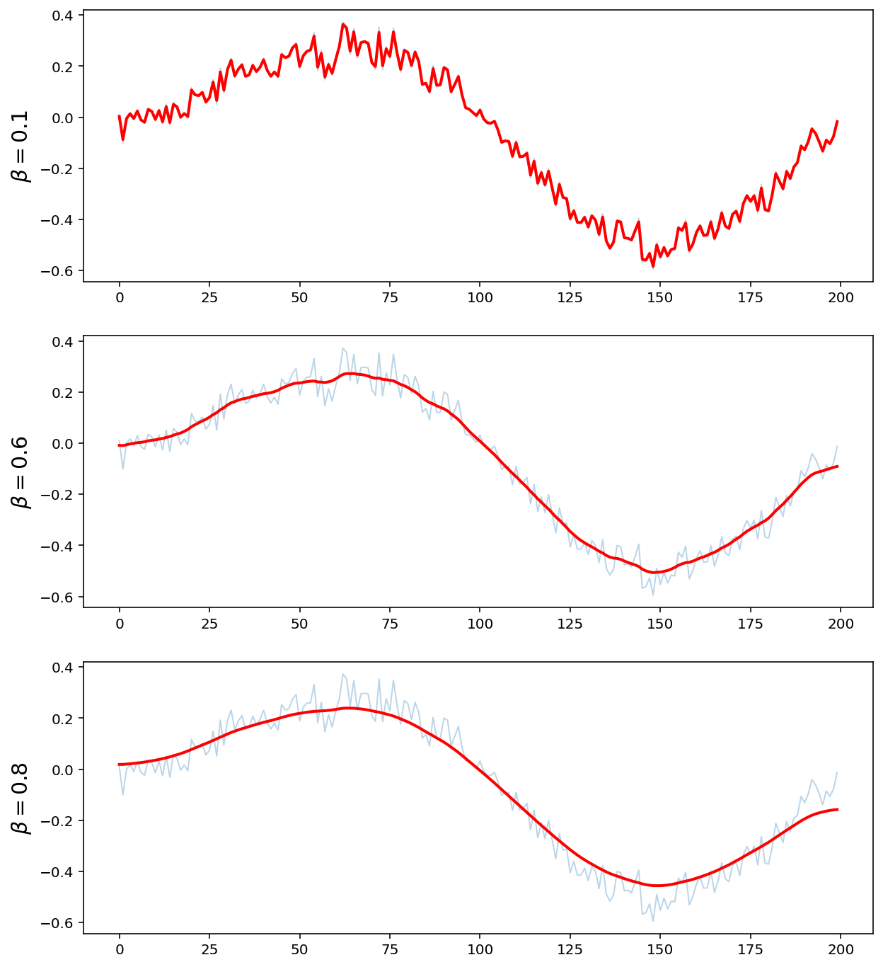
1.5. L2 Norm with a Constraint
\(\min \; \lVert Dx \rVert_2\) \(\text{s.t.} \quad \lVert x-x_{cor} \rVert_2 < \beta\)
beta = 0.8

x_reconst = cvx.Variable([n,1])
obj = cvx.Minimize(cvx.norm(D*x_reconst, 2))
const = [cvx.norm(x_reconst-x_cor, 2) <= beta]
prob = cvx.Problem(obj, const).solve()

plt.figure(figsize = (10, 4))
plt.plot(t,x_cor,'-', linewidth = 1, alpha = 0.3)
plt.plot(t,x_reconst.value, 'r', linewidth = 2)
plt.ylabel(r'$$\beta = {}$$'.format(beta), fontsize = 15)
plt.show()
plt.figure(figsize = (10, 12))

beta = [0.1, 0.6, 0.8]

for i in range(len(beta)):

    x_reconst = cvx.Variable([n,1])
    obj = cvx.Minimize(cvx.norm(x_reconst[1:n] - x_reconst[0:n-1], 2))
    const = [cvx.norm(x_reconst-x_cor, 2) <= beta[i]]
    prob = cvx.Problem(obj, const).solve()

    plt.subplot(len(beta),1,i+1)
    plt.plot(t,x_cor,'-', linewidth = 1, alpha = 0.3)
    plt.plot(t,x_reconst.value, 'r', linewidth = 2)
    plt.ylabel(r'$$\beta = {}$$'.format(beta[i]), fontsize = 15)

plt.show()
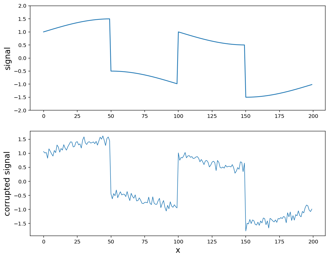
2. Signal with Sharp Transition + Noise
Suppose we have a signal \(x\), which is mostly smooth, but has several rapid variations (or jumps). If we apply quadratic smoothing on this signal, then in order to remove the noise we will not be able to preserve the signal’s sharp transitions.
- First, apply the same method that we used for smoothing signals before.
n = 200
t = np.arange(n).reshape(-1,1)

exact = np.vstack([np.ones([50,1]), -np.ones([50,1]), np.ones([50,1]), -np.ones([50,1])])
x = exact + 0.5*np.sin((2*np.pi/n)*t)
x_cor = x + 0.1*np.random.randn(n,1)

plt.figure(figsize = (10, 8))
plt.subplot(2,1,1)
plt.plot(t, x)
plt.ylim([-2.0,2.0])
plt.ylabel('signal', fontsize = 15)
plt.subplot(2,1,2)
plt.plot(t, x_cor, linewidth = 1)
plt.ylabel('corrupted signal', fontsize = 15)
plt.xlabel('x', fontsize = 15)
plt.show()
2.1. L2 Norm (Quadratic Smoothing)
plt.figure(figsize = (10, 12))

beta = [0.5, 2, 4]

for i in range(len(beta)):
    x_reconst = cvx.Variable([n,1])
    obj = cvx.Minimize(cvx.norm(x_reconst[1:n] - x_reconst[0:n-1], 2))
    const = [cvx.norm(x_reconst - x_cor, 2) <= beta[i]]
    prob = cvx.Problem(obj, const).solve()

    plt.subplot(len(beta), 1, i+1)
    plt.plot(t, x_cor, linewidth = 1, alpha = 0.3)
    plt.plot(t, x_reconst.value, 'r', linewidth = 2)
    plt.ylabel(r'$$\beta = {}$$'.format(beta[i]), fontsize = 15)

plt.show()
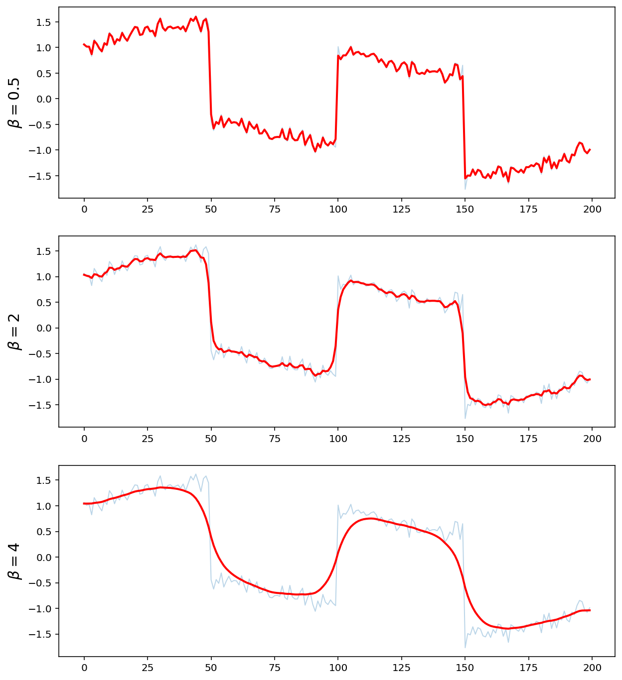
-
Quadratic smoothing smooths out noise and sharp transitions in signal, but this is not what we want
-
Any ideas ?
2.2. L1 Norm
We can instead apply total variation reconstruction on the signal by solving
\(\min \; \lVert x - x_{cor} \rVert_2 + \lambda \sum_{i=1}^{n-1} \;\lvert x_{i+1}-x_i \rvert\) where the parameter \(\lambda\) controls the ‘‘smoothness’’ of \(x\).
\(\min \; \lVert Dx \rVert_1\) \(\text{s.t.} \quad \lVert x-x_{cor} \rVert_2 < \beta\)
plt.figure(figsize = (10, 12))

beta = [0.5, 2, 4]

for i in range(len(beta)):
    x_reconst = cvx.Variable([n,1])
    obj = cvx.Minimize(cvx.norm(x_reconst[1:n] - x_reconst[0:n-1], 1))
    const = [cvx.norm(x_reconst-x_cor, 2) <= beta[i]]
    prob = cvx.Problem(obj, const).solve()

    plt.subplot(len(beta), 1, i+1)
    plt.plot(t, x_cor, linewidth = 1, alpha = 0.3)
    plt.plot(t, x_reconst.value, 'r', linewidth = 2)
    plt.ylabel(r'$$\beta = {}$$'.format(beta[i]), fontsize = 15)

plt.show()
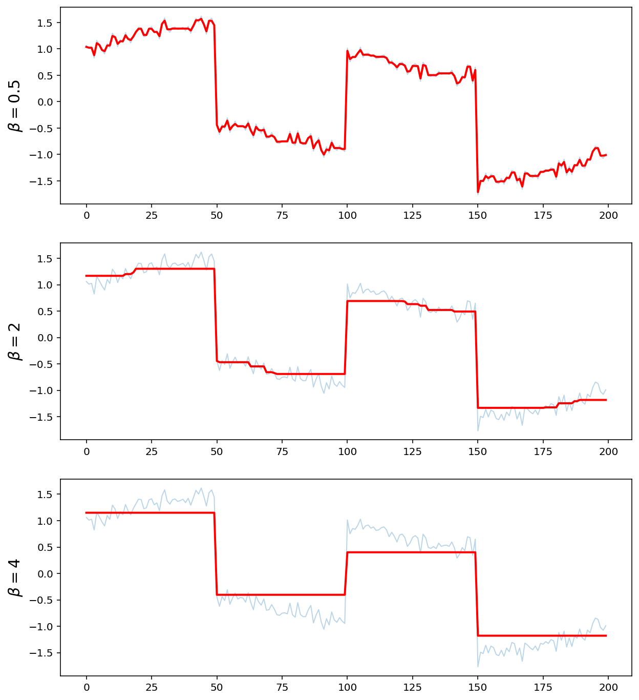
-
Total Variation (TV) smoothing preserves sharp transitions in signal, and this is not bad
-
Note how TV reconstruction does a better job of preserving the sharp transitions in the signal while removing the noise.
3. Total Variation Image Reconstruction
import cv2

imbw = cv2.imread('bird.bmp', 0)

row = 150
col = 150
resized_imbw = cv2.resize(imbw, (row, col))

plt.figure(figsize = (8,8))
plt.imshow(resized_imbw, 'gray')
plt.axis('off')
plt.show()
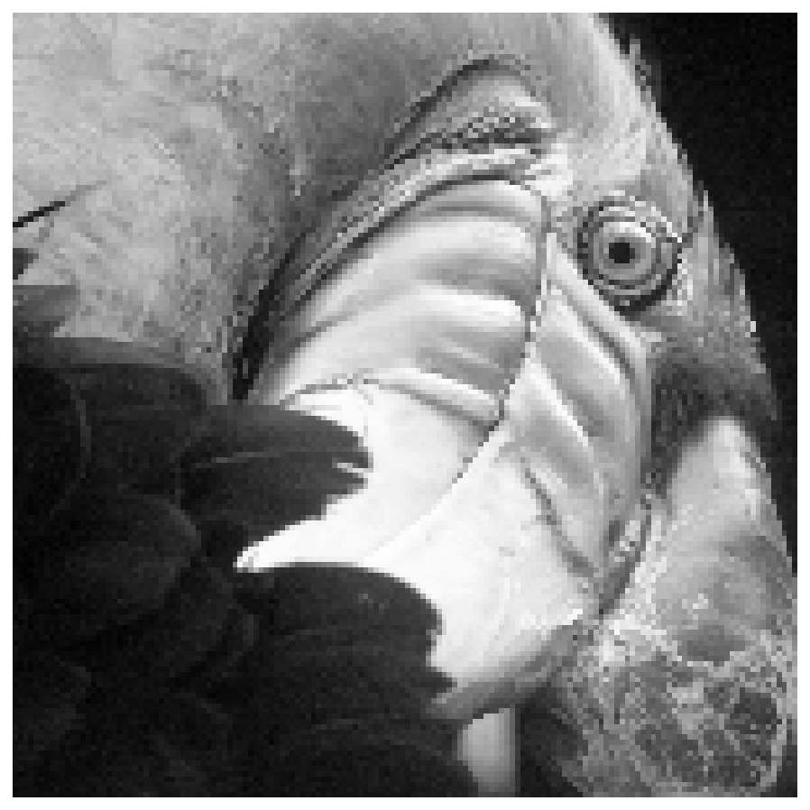
- Question: Apply \(L_1\) norm to the image, and guess what kind of an image will be produced ?
\(\min \; \lVert Dx \rVert_1\) \(\text{s.t.} \quad \lVert x-x_{cor} \rVert_2 < \beta\)
n = row*col
imbws = resized_imbw.reshape(-1, 1)

beta = 1500

x = cvx.Variable([n,1])
obj = cvx.Minimize(cvx.norm(x[1:n] - x[0:n-1],1))
const = [cvx.norm(x - imbws,2) <= beta]
prob = cvx.Problem(obj, const).solve()

imbwr = x.value.reshape(row, col)

plt.figure(figsize = (8,8))
plt.imshow(imbwr,'gray')
plt.axis('off')
plt.show()
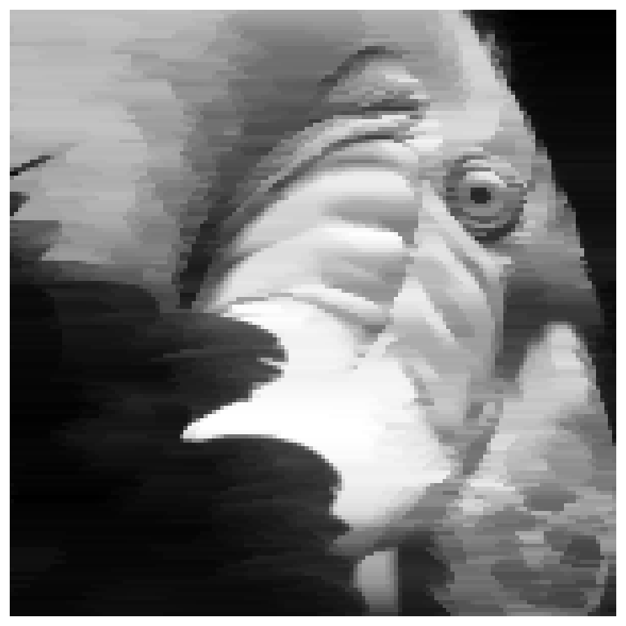
- Cartoonish effect
Leave a comment