Pathfinding in Pacman domain

Introduction

Pathfinding builds on top of graph search algorithms and explore routes between nodes, traversing from the start node to the destination. These algorithms are used to identify optimal routes through a graph for uses such as logistics planning (Vehicle routing/logistics), least cost call or IP routing, and gaming simulation (AI movements or user assistance). The following figures are applications of pathfinding; logistics planning, robotics, and game-playing.

I applied pathfinding to Pacman domain (gaming-play application) to compare which algorithms are suitable in the case.

Graphs

A graphs can represent networks of communication, data organization, computational devices, the flow of computation, etc, depending on how you set up nodes and edges.

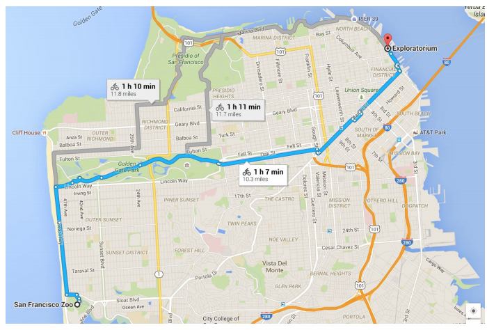
For instance, we can set an input as a graph of the map like a set of locations (nodes) and the connections (edges) can be input. The following figures shows how a map is represented as a graph. The shaded path is the shortest path in the graph, the blue dots are nodes, and the green lines are edges.

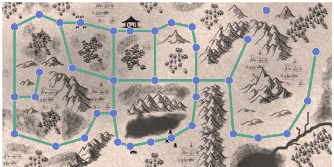
| Fig1. Applications of pathfinding |

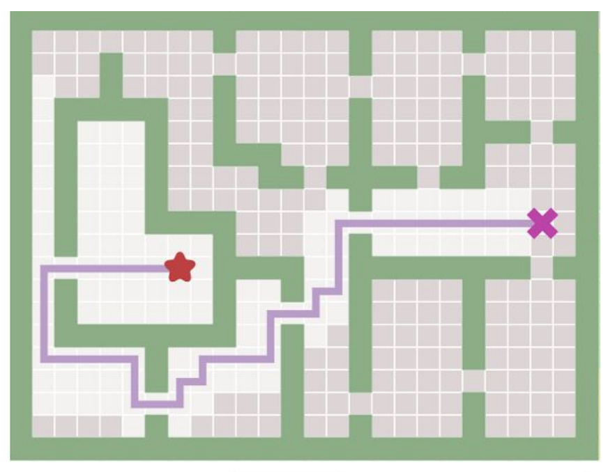
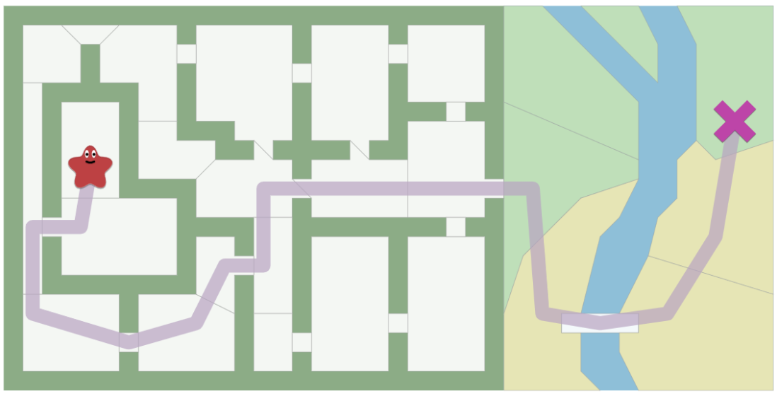
This map can represent in many different ways. One can be doorways as edges (left in the Fig2) or another can be a grid mapping.

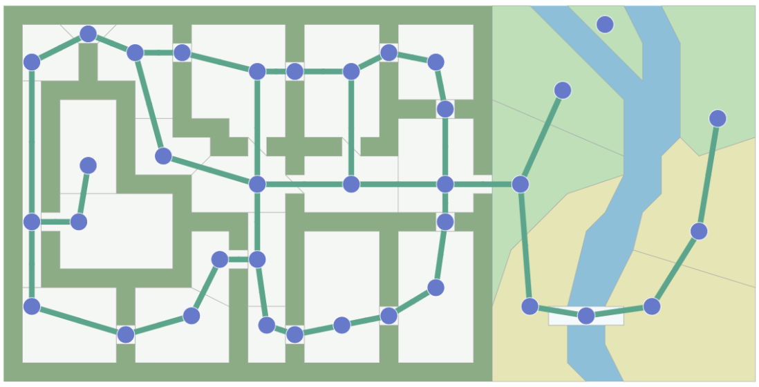
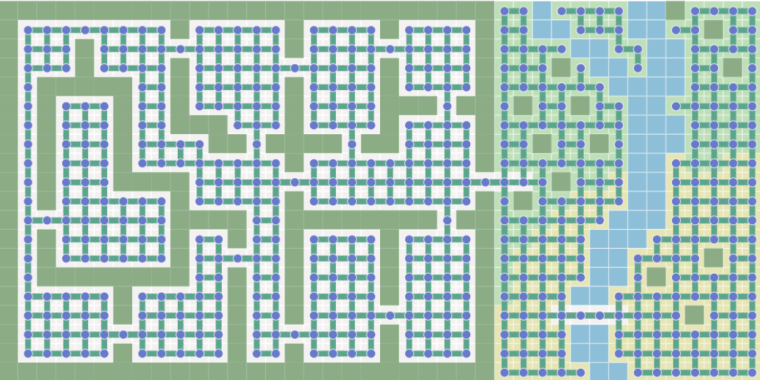
| Fig2. The map represented as a graph|

A pathfinding graph can vary, depending on how you define. In the Pacman domain, the map is designed as a grid.

Shortest Path

The Shortest Path algorithm calculates the shortest (weighted) path between a pair of nodes. One of the most popular shortest path algorithms is Dijkstra’s.

NOTE Dijkstra’s is known as Uniform Cost Search.

The goal of this project is to see how the behaviors of graph search algorithms in the Pacman domain and how heuristic affects them while finding the shortest path.

** NOTE** You can think of heuristic an approximate measure of how close you are to the target.

Fig3 shows pathfinding of Bi-directional search in the Pacman domain. Unlike an Uni-directional search that explores nodes from only departure, a Bi-directional search explores starting from both departure and destination.

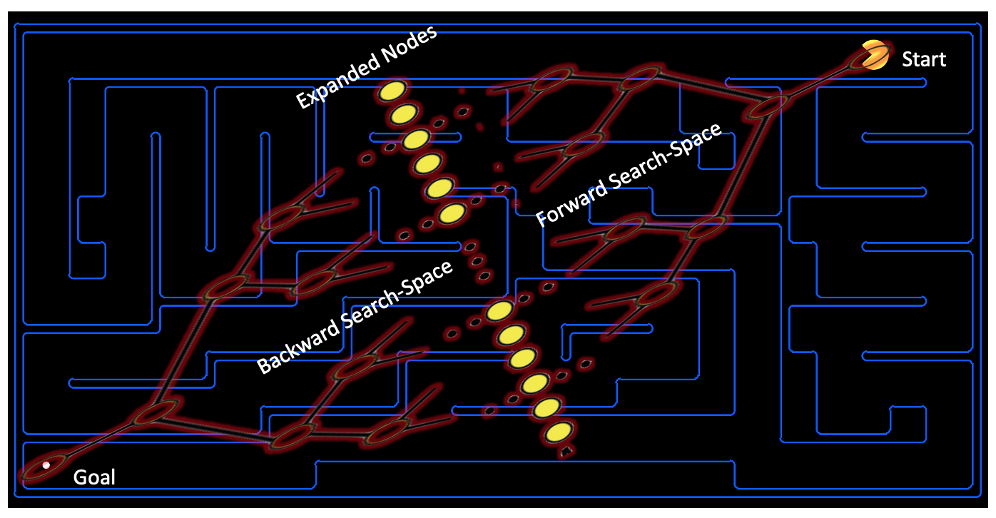
| Fig3. Bi-directional Pathfinding in Pacman Domain |

Blind Searches vs Heuristic Searches

There are various search algorithms, but we can categorize them into two: blind searches and heuristic searches.

The following video shows how BFS and UCS search to the goal location. Their final paths are different cause blind searches don’t take edge weights into account; they don’t care about the edge is weighted or not.

NOTE You don’t want to consider a flooded path to be the same as a ground path. So concept of ‘weight’ is introduced to each path (edge).

A BFS explores around the departure whereas an UCS explores toward the destination and ignores some of unnecessary nodes. That is because of heuristic estimation. Intuitively, heuristic can reduce computational time of exploring nodes.

| Fig4. Heuristic Searches vs Blind Searches |

Bi-directional Search

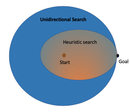
Similarly, Bi-directional searches helps reducing exhaustive exploring even without using a heuristic.

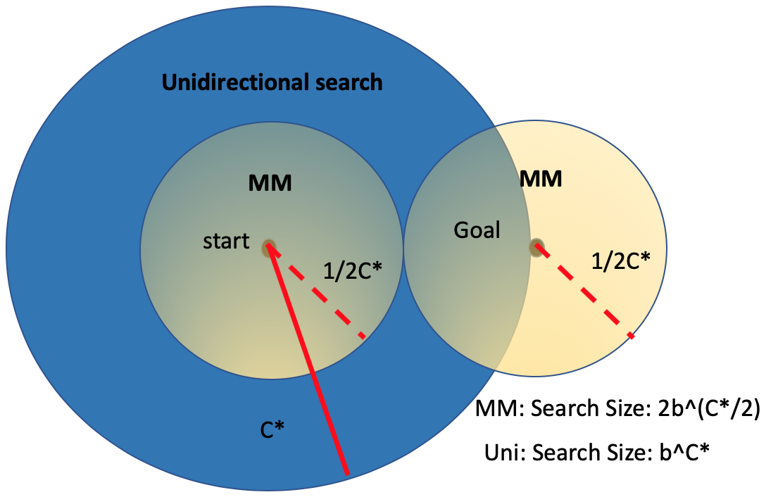
| Fig5. Bi-directional Searches without a Heuristic |

In this project, BFS (Breadth-First Search), DFS (Depth-First Search), A* (A* Search), USC (Uniform Cost Search), and BiS (Bi-directional Search) are applied to Pacman domain to know which search algorithm performs best.

If you are not familiar with those algorithms, check this tutorial. Also, you can play with this to understand how each search algorithm work.

Bi-directional Search Type

Fig6 shows BiS types.

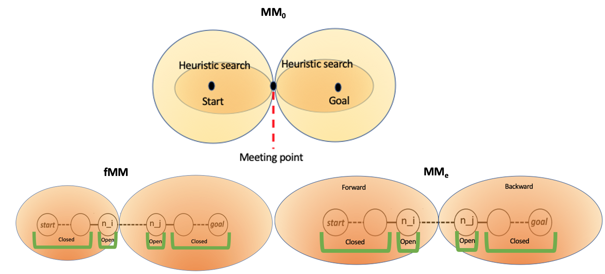
| Fig6. Bi-directional Search Type |

1. \(MM_0\): BiS without heuristic. There are forward search (from departure) and backward search (from destination). MM means ‘M’eet in the ‘M’iddle.

2. \(MM_{\epsilon}\): It is also a blind search, but covers the case that an optimal path is yet found. Using a priority (heuristic) function for both forward search and backward search, stretching the exploration to cover the gap between two explore regions.

3. \(fMM\): Fractional MM doesn’t necessarily meet at the middle; it can fractionally decide which explore region should be bigger. It means that explore regions between forward search and backward search have different size, depending on the graph.

Demo / Conclusion

The following video is the demo of how DFS and BiS with Manhattan heuristic find their optimal paths.

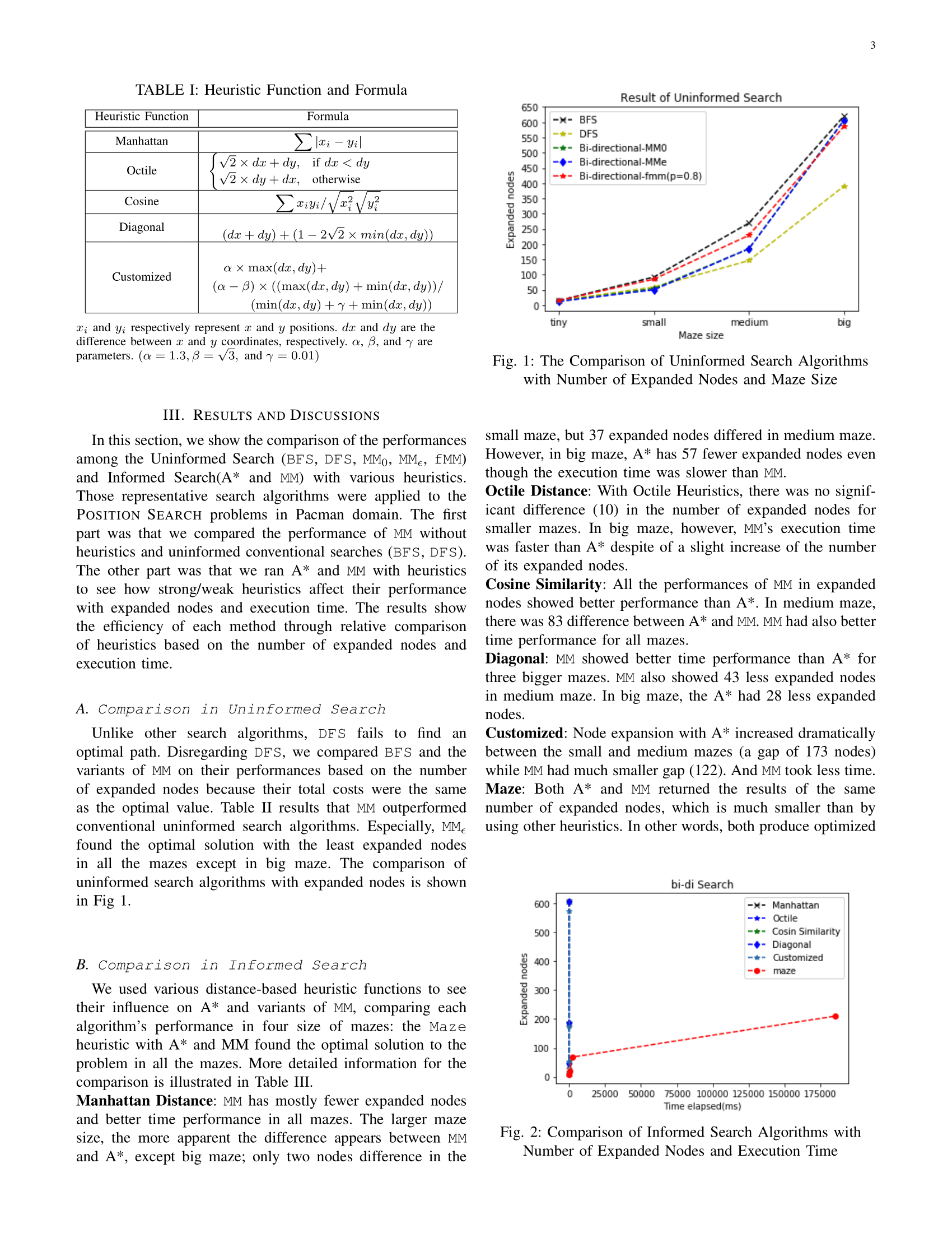
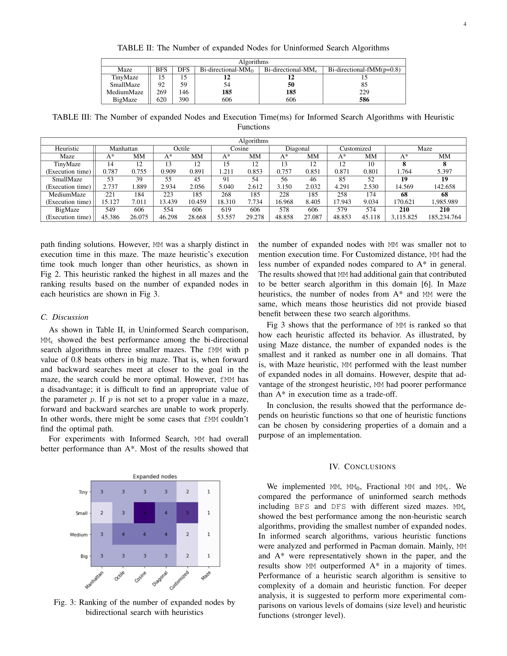
Even though BFS and DFS are included, \(MM_{\epsilon}\) showed the best performance among the blind searches. For heuristic searches, MM outperformed A* in a majority of times. Performance of a heuristic search is sensitive to complexity of the Pacman domain and heuristic function.

If you are interested in more detail code and theory, please check my github and my paper shown below.